Web Handling Training with MapleSim

Web-based manufacturing is one of the essential but often unseen foundations of modern industry. Every day, enormous quantities of material-films, papers, foils, textiles, nonwovens, composites, and laminates move through machines as continuous flexible sheets known as webs. These webs are converted into the packaging we open, the medical products we rely on, the electronics we use, and the energy-storage materials that power emerging technologies.
This chapter introduces the core concepts of web handling, establishing the framework for the training that follows. It defines what a web is, explains why web handling is foundational, outlines the key machine elements, and highlights the role of dynamic simulation in designing and improving converting lines.
A web is a continuous, flexible sheet of material transported through a manufacturing process where the web may be printed or coated, laminated, embossed, folded, slit or die cut, and often wound on a roll. Before being converted, webs are first created in processes such as papermaking, film extrusion, fiber spinning, or metal rolling. Webs are generally characterized by being very thin relative to their width and length.
Examples include:
• Plastic films such as polyethylene, polypropylene, and PET
• Paper, paperboard, and specialty papers
• Aluminum foil and metallized films
• Adhesive tapes and label stock
• Nonwovens used in hygiene, filtration, and medical products
• Battery separator films and electrode coatings
• Textiles, technical fabrics, and composite prepregs
Regardless of the material, webs must be transported under controlled tension, position, and dimensional stability to avoid damage to webs or machine components, and unplanned machine stops.

Web converting encompasses the processes that transform raw web materials into finished or semi-finished products. It is a broad, multi-industry discipline that includes:
Because converting lines integrate many value-adding steps, the stability and quality of web transport directly influence the performance of every downstream process.
Web handling is an engineering discipline focused on transporting a web through a web-making or converting process without damage, loss of control, quality degradation, or unplanned machine stops. It ensures that the web arrives at each process step in the necessary state, both in steady-state and dynamic conditions:
When web handling is unstable, defects such as wrinkles, curl, misregistration (incorrect MD/CD position), scratches, baggy lanes, and web breaks may occur. Many converting problems trace back to fundamental handling issues in addition to the converting processes that interact with the web's transport.
A web's mechanical properties determine how it behaves under tension, over rollers, and through dynamic changes in the line. Key properties include:
Understanding these properties and including them in process simulations helps web converters anticipate challenges such as wrinkles, slip, curl, or tension nonuniformity.
Most web-handling systems share a common architecture:
The web is unwound from a roll. Tension is controlled using brakes, motors, or dancer systems or load cells and roll diameter sensors that function together to compensate for roll-diameter changes and disturbances.
The web travels over a sequence of rollers separated by free spans. Each roller guides, supports, or isolates tension. Spans behave like tensioned membranes and are sensitive to vibration, alignment, and tension changes.
The finished web is rewound under controlled tension and nip conditions to produce a stable, defect-free roll.
A "web path" is created by the sequence of rollers, spans, and converting processes that the web follows to its final state.
This architecture appears simple, but the dynamic interactions between rollers, drives, tension loops, and the web itself create a complex system requiring careful design and control.
Rollers are central to web transport. Common types include:
The optimal number of idlers, driven rollers, and specialty rollers and their placement in a web path needs analysis when designing or modifying a web transport system.

Spans are the open spaces between rollers that the web takes on its path through the machine. They allow the web to transition between rollers. Their length, tension, and alignment affect wrinkle formation, vibration, and lateral stability. It is a balance to design a web path with the right number of rollers and span lengths to optimize the capital cost of equipment, web handling process reliability and product quality.
These parts of the web line define the entry and exit of the converting line. Their control systems must adapt to changing roll diameters, inertia, and winding stresses.
Unwinds help deliver the web from a wound roll into the converting process and winders convert a transformed web into a single wound roll or multiple rolls after slitting. Unwinds often include splicing operations to join the end of an expiring roll to the start of a new roll, and many designs of winders include the ability to start winding new rolls after the previous roll has completed winding.
Since tension on the web impacts so many things about its proper handling, various tension control methods are used in web converting lines:
Together, these components form the tension loops that define the web's mechanical state throughout the line.
Small imperfections in rollers can create significant process disturbances:
Identifying and mitigating these issues is essential for stable operation.
Multiple webs are combined using heat, pressure, or adhesive. Strain matching at the combining point is critical to avoid curl, bubbles, and wrinkles.
A wide web is cut into narrower rolls or edge trim lanes are removed from a web. There are shear slitters, crush slitters, knife blade slitters and even laser or water jet slitters used in slitting operations. Tension control of the web at any slitting operation is essential to maintaining slit width and slit edge quality.
Other processes-coating, printing, drying, embossing, calendering-each impose their own mechanical constraints, all of which depend on stable web handling.
Modern converting lines are complex dynamic systems. Dynamic simulation provides a powerful way to understand and optimize their behavior. It enables:
Simulation reveals tension oscillations, roller dynamics, and control interactions that are difficult or impossible to measure directly, making it a critical tool for modern web-handling engineering.
The remainder of this training will introduce you to MapleSim and the Web Handling Library and show you how to apply this simulation tool in the design and improvement of web transport systems.
Web handling is the foundation upon which all web converting rests. A deep understanding of web behavior, machine dynamics, and tension control enables engineers to design better systems, troubleshoot complex problems, and improve product quality. This training program builds from these fundamentals toward a practical, simulation-supported mastery of web-handling principles.
Introduction to Modeling with MapleSim
MapleSim is a multidomain system-level modeling and simulation tool that enables users to perform dynamic simulations across various domains using built-in libraries. These domain’s include Web Handling, Electrical, Multibody, Hydraulics, Pneumatics, and more. To build dynamic models in MapleSim, users must first become familiar with the environment. This chapter focuses on understanding the MapleSim interface, constructing a simple model using library components, exploring key features for model setup, and running simulations.
In this section, we will explore the MapleSim interface and gain a comprehensive understanding of the various features and functionalities available to users. To begin with we will discuss on the different modeling components, parameter configurations, and simulation settings that are essential for constructing a well-defined system model.Furthermore, we will explore options such as configuring solver settings, and modifying the simulation parameters for better performance.
Finally, we will dwelve into the post-processing capabilities of MapleSim which includes looking into our Result manager window where a user can look at the results such as plots/3D model to gain valuable insights into their system’s behavior and refine their models accordingly if need be.
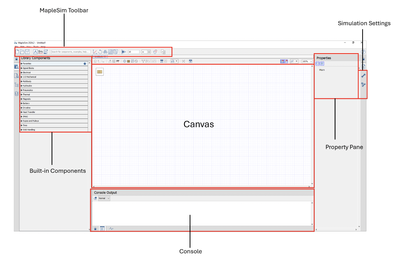
Figure 1.1: MapleSim Interface
The MapleSim canvas serves as the primary workspace within the tool, allowing users to drag and drop components from the library to construct their models. The placement of components on the canvas is purely for visual organization and does not influence the actual simulation.
While users have the flexibility to position components anywhere within the canvas, the physical behavior of the model is determined by the connections between components and the port information. These connections define how different elements interact and ultimately influence the simulation results.
MapleSim’s component library contains more than hundreds of pre-built components that can be used to build models. These components are catogorized into different domains making it easier to navigate and quick selection of the most suitable components for a given application. Furthermore, users are not restricted to the built-in components available in the library. MapleSim provides the flexibility to create custom components, enabling users to tailor models to their specific needs. This capability will be explored in detail in a later session.
MapleSim toolbar provides a range of essential tools that can help the user with their modeling workflow. It allows users to:
Run simulations to test and analyze their models.
View and interpret simulation results through built-in result manager window.
Perform reruns to refine model performance and troubleshoot issues
Import external files, such as CAD models and Functional Mock-up Units (FMUs), to integrate with existing designs
Open a Maple worksheet enabling advanced custom post-processing.
Access built-in applications that provide additional functionalities to enhance model development and post-processing.
The simulation settings provide users with the ability to configure various aspects of their model setup.
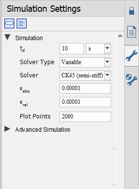
Figure 1.2: Simulation Settings
These settings allow users to:
Adjust the simulation duration to match the requirements of their analysis.
Select the most appropriate solver type based on the specific application needs.
Define the minimum number of data points to be plotted for accurate result visualization.
Import external files, such as CAD models and Functional Mock-up Units (FMUs), to integrate with existing designs
Set error tolerances to ensure numerical stability and precision in the results.
The Advanced Settings provide additional configuration options for a more detailed model setup
The Console Output presents progress messages that reflect the status of the MapleSim engine during simulation. Additionally, it provides details on model failures and warnings, helping users diagnose and troubleshoot issues effectively.
In this section, we will walk through the process of building a planar double-pendulum model in MapleSim, utilizing the primitives section of the Web Handling Library. The goal of this chapter is to guide the user in creating a simple model by effectively using the interface options discussed in the previous sections. While we will focus on the basic implementation of the model here, a more in-depth introduction to the components from the Web Handling Library will be provided in a subsequent chapter. The primitives section of the Web Handling (WH) Library consists of specialized multibody-based components designed to accurately position the web handling elements within a model. These components, much like the other elements found in the Web Handling Library, are restricted to a two-dimensional plane, specifically the x-y plane.
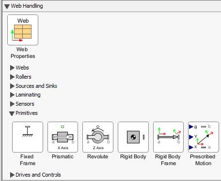
Figure 1.3: Primitives section-WH Library
The schematic of a double pendulum model is shown below:
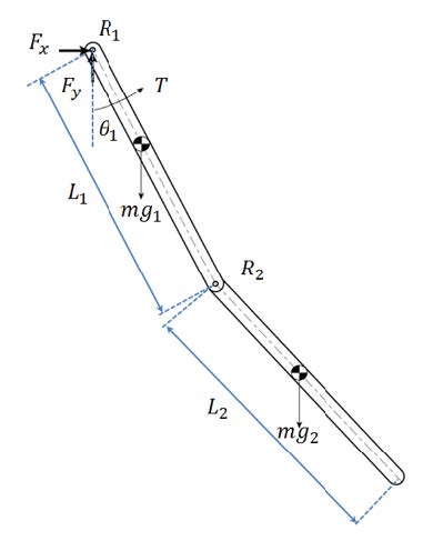
Figure 1.4: Double pendulum mechanism
This model consists of a revolute joint, R1, which is attached to the first planar link. This planar link is attached to the second planar link through a second revolute joint, R2. For the system shown in the diagram, gravity is assumed to be the only external force, acting along the negative y-axis.
However, it is advisable to follow the steps below to construct the model from scratch. The figure below provides an overview of the model that will be built in this section:
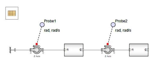
Figure 1.5: Double Pendulum Model
Use the following steps to create the model in MapleSim:
Open a new MapleSim document and save it as “Double_Pendulum.msim”
Under the Libraries tab, browse to the Web Handling > Primitives menu, and then add two Rigid Body Frame components and a Rigid Body component.
Drag the components in the arrangement shown below and connect the components together by drawing connection lines between the RB and RBF components.
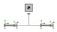
Figure 1.6: Creating a linkage in MapleSim
Select all the three components and right-click. From the context menu, select ‘Create Subsystem’. In the subsystem dialog box, enter ‘Link’, and then click ‘OK’.
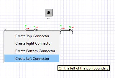
Figure 1.7: Connecting component to subsystem boundary
In this task, you will define a subsystem parameter, L, to represent the length of the link and assign the parameter value as a variable to the parameters of the Rigid Body Frame components. The Rigid Body Frame components will then inherit the numeric value of L.
To define and assign parameters:
Double-click on the ‘Parameters View’ (![]() ) to display the subsystem default settings. In the first row, define a parameter called L and press ‘Enter’. Specify ‘Length’ for ‘Type’, 1 for ‘Default Value’, ‘m’ for ‘Default Units’, and ‘Length’ for ‘Description’ as follows:
) to display the subsystem default settings. In the first row, define a parameter called L and press ‘Enter’. Specify ‘Length’ for ‘Type’, 1 for ‘Default Value’, ‘m’ for ‘Default Units’, and ‘Length’ for ‘Description’ as follows:
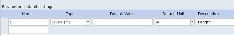
Figure 1.8: Define Link parameters
Click ‘Diagram View’ (![]() ) in the Navigation Toolbar to go back to the diagram view.
) in the Navigation Toolbar to go back to the diagram view.
Select both of the Rigid Body Frames simultaneously by pressing ‘Ctrl’ and then selecting each of the components. Specify the common parameter ˜r to be [L/2, 0, 0] [m].
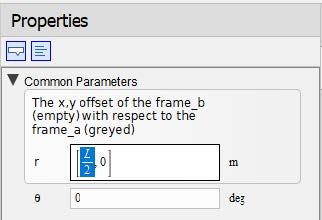
Figure 1.9: Define common parameters
Click ‘Return to Main’ (![]() ) located in the top left corner in the Navigation Toolbar to go back to the main level of the model.
) located in the top left corner in the Navigation Toolbar to go back to the main level of the model.
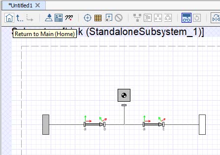
Figure 1.10: Return to Home
To create the double pendulum mechanism, follow these steps:
Right-click on the Link subsystem and select ‘Convert to a Shared Subsystem’
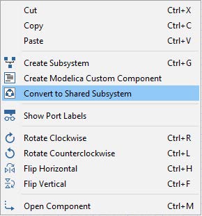
Figure 1.11: Right-click menu
Enter ‘Link’ in the pop-up menu:
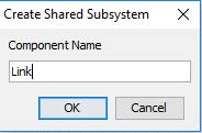
Figure 1.12: Enter the name for the shared subsystem
Click ‘OK’.
Under the ‘Library Components’ tab (![]() ), drag a Fixed Frame component and a Revolute from Web Handling > Primitives menu.
), drag a Fixed Frame component and a Revolute from Web Handling > Primitives menu.
Click the subsystem Link2 , enter 2 for the parameter L.
Connect the components and subsystems together as shown in the following diagram:
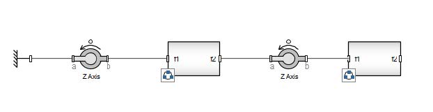
Figure 1.13: Double Pendulum
To simulate the model and observe the simulation results:
From the Model Workspace Toolbar, click ‘Attach Probe’ (![]() ).
).
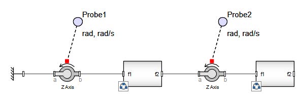
Figure 1.14: Adding probes
Click ‘Run Simulation’ (![]() ) in the Main Toolbar (or hit ‘F5’). When the simulation is complete, the following plots appear:
) in the Main Toolbar (or hit ‘F5’). When the simulation is complete, the following plots appear:
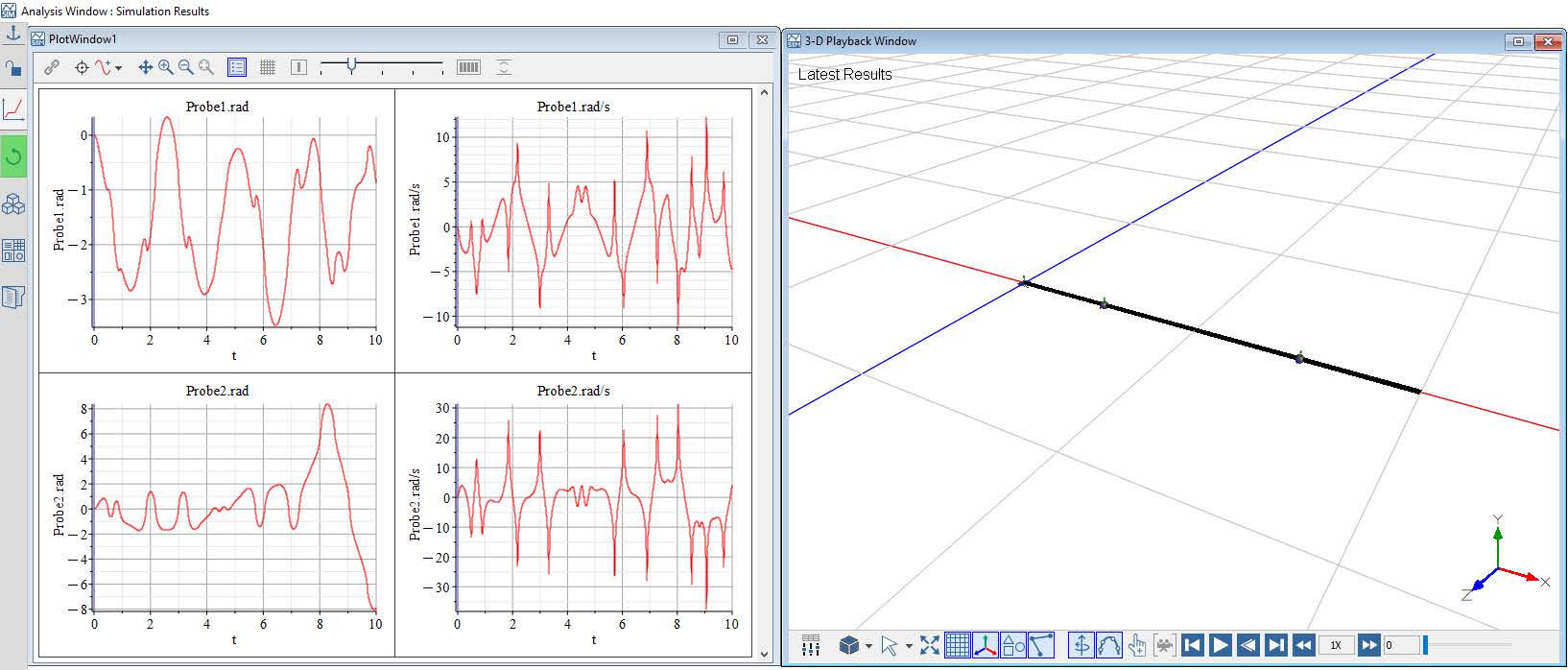
Figure 1.15: Simulation results
Click ‘Play’ (![]() ) in the 3-D Playback Window to see an animation of the simulation results.
) in the 3-D Playback Window to see an animation of the simulation results.
Using components from the Multibody mechanical library, you will model the planar slider-crank mechanism shown in the following figure:
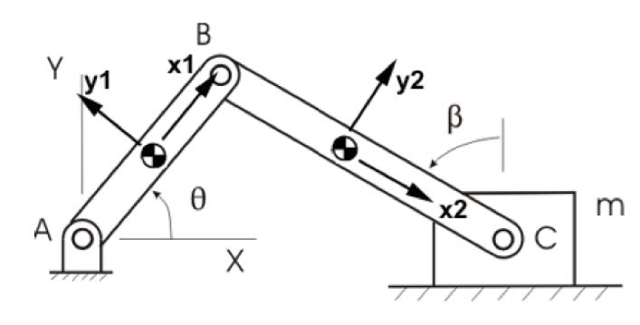
Figure 1.16: Planar slider-crank mechanism
However, it is advisable to follow the steps below to construct the model.
The figure below provides an overview of the model that will be built in this section:
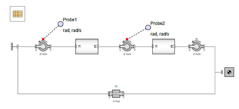
Figure 1.17: Slider Crank Model
The slider-crank mechanism can be created by expanding the double-pendulum example created in the previous section.
Open the “Double_Pendulum.msim” model from the previous section and save it as “Slider_Crank.msim”.
Drag a Rigid Body , a Revolute and a Prismatic component from the Web Handling > Primitives menu.
Connect the components together using the above arrangement.
Click ‘Run Simulation’ (![]() ) in the Main Toolbar (or hit ‘F5’). When the simulation is complete, the following plots appear:
) in the Main Toolbar (or hit ‘F5’). When the simulation is complete, the following plots appear:
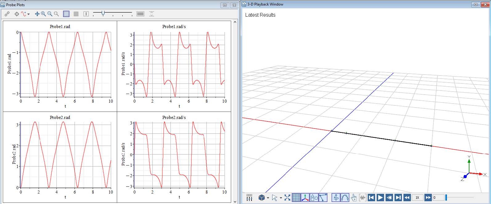
Figure 1.18: Unactuated Slider Crank
This simulation shows the results of an actuation slider crank mechanism. Now lets add an actuation to the model.
In this section, we will introduce a basic actuation mechanism to the model by briefly exploring the 1D Mechanical Library in MapleSim. This will provide an initial understanding of how actuation can be implemented within the system. While this section offers a quick overview, a more in-depth exploration of actuation techniques, control strategies, and their impact on system behavior will be covered in the upcoming sections.
The figure below provides an overview of the model that will be built in this section:
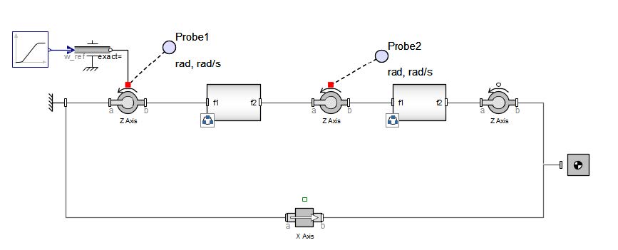
Figure 1.19: Actuated Slider Crank Mechanism
Drag a Rotational Speed component from 1-D Mechanical > Motion Drivers menu. This component enerates a forced angular speed according to the input signal its connected to.
For the input signal, we are going to bring in a Ramp component from Signal Blocks > Common menu.
Use the following settings for the Ramp component.
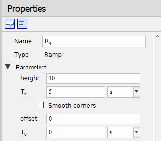
Figure 1.20: Ramp parameters
Make the connection as shown in the above.
Click ‘Run Simulation’ (![]() ) in the Main Toolbar (or hit ‘F5’). When the simulation is complete, the following plots appear:
) in the Main Toolbar (or hit ‘F5’). When the simulation is complete, the following plots appear:
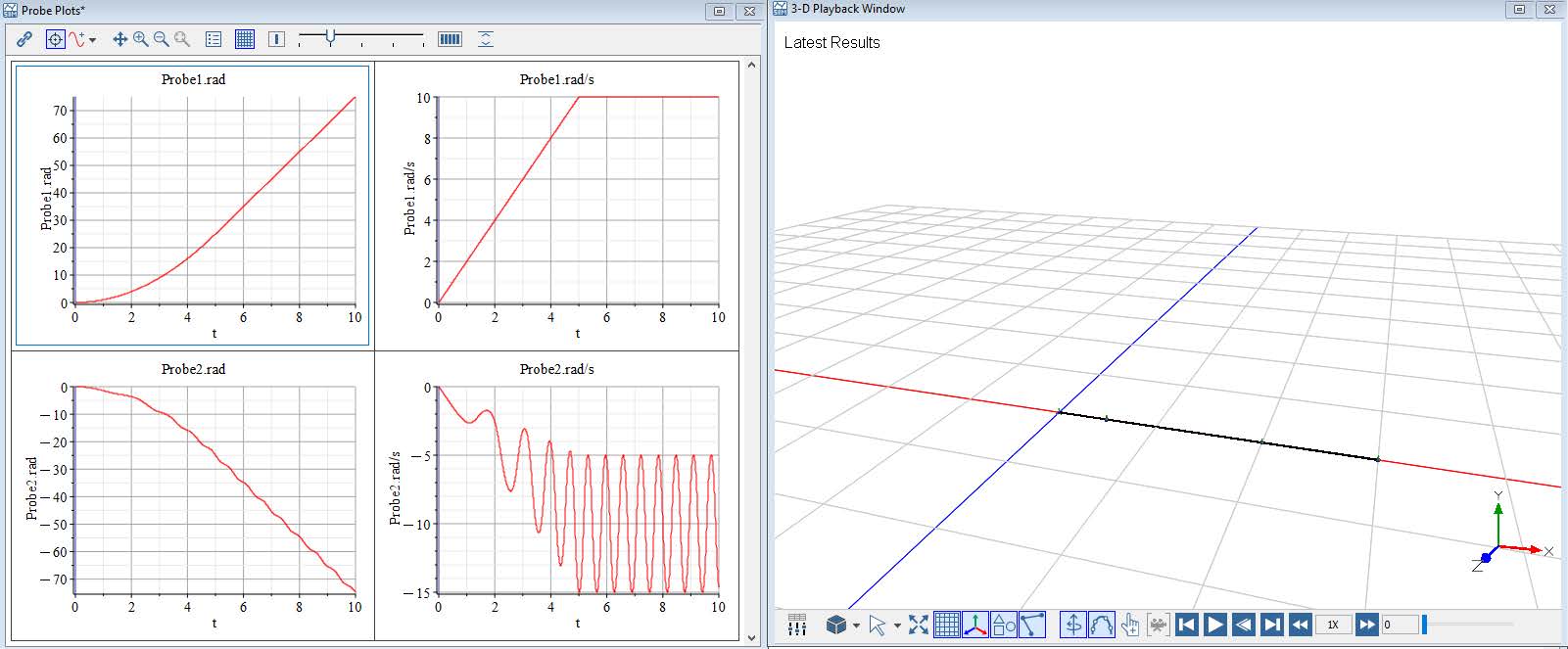
Figure 1.21: Actuated Slider Crank Results
Press the simulation play back button to visualize the simulation.
The Primitives subsection of the Web Handling Library which is used to build simple planar mechanism in this chapter is actually a subset of a much elaborate Multibody Library in MapleSim. If interested one can look into the Multibody Library which is specifically created to model 3-D multibody mechanical systems in MapleSim.
Introduction to Web Handling Library
Let us take a moment to briefly discuss the various components available within the Web Handling Library. Compared to other libraries in the tool, the Web Handling Library offers a more straightforward and intuitive experience for users, particularly when it comes to building and understanding system models. One of the key reasons for its user-friendliness is its planar modeling approach, which restricts the system to two dimensions—making it easier to visualize and comprehend. Additionally, the components in this library come with clear visual representations and built-in animations, which help users quickly grasp the physical behavior of the system and validate model functionality in a more interactive manner. Lets now look into the major categories of the library.
Lets look into the various sub-categories of the library components.
Web Properties
Webs
Rollers
Sources and Sinks
Laminating
Slitting
Sensors
Primitives
Routing
Drives and Controls
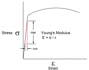
The Web Properties block allows users to define the mechanical and physical characteristics of the web material used in their model. This includes essential parameters such as width, thickness, density, Young’s modulus (elastic modulus), and Poisson’s ratio—all of which directly influence the dynamic behavior of the web during operation.
In addition to the mechanical properties, this block also enables users to configure the visualization settings for the web, allowing for clearer and more informative animations during simulation. This block is a record where the properties automatically apply to all components located at the same hierarchical level or within any subsystems below it. Moreover, each components from the library includes a field to reference a specific Web Property block. This allows models to incorporate multiple web types by assigning the appropriate Web Property block to each corresponding component.
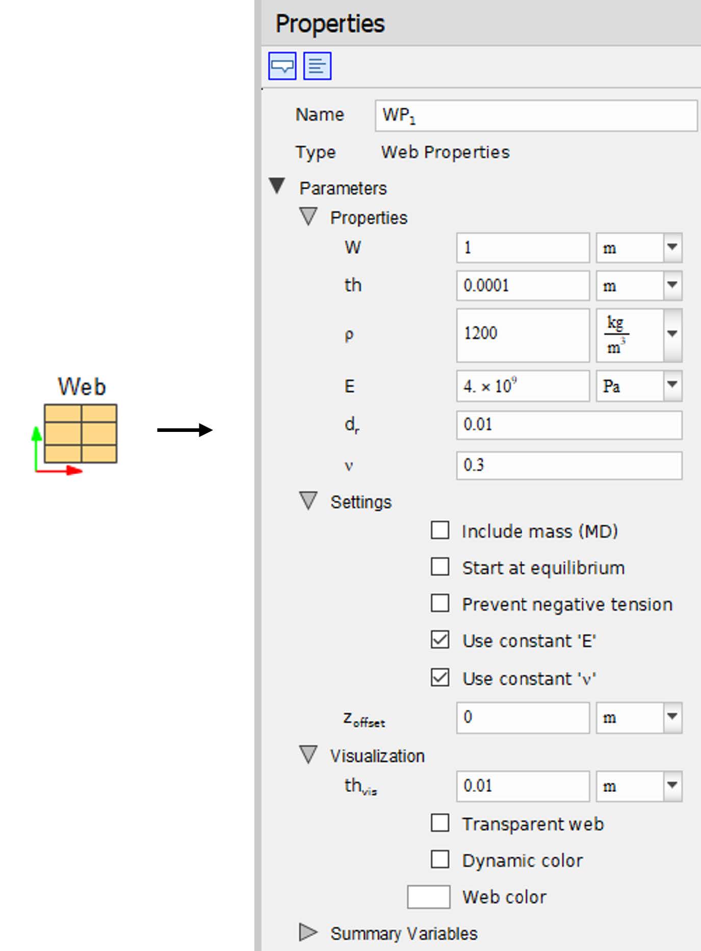
Figure 2.1: Web Property Block
Nonlinear Material - Variable Modulus of Elastisity - When the Use constant ’E’ option is unselected, new parameters are enabled to define the modulus of elasticity as a function of strain via a lookup table.
Nonlinear Material - Variable Poisson’s Ratio - When the Use constant "’nu’"option is unselected, new parameters are enabled to define the Poisson’s ratio as a function of strain via a lookup table.
Include Mass (Machine Direction) - When the Include Mass (MD) option is selected, all spans in the model activate a second equation for the conservation of momentum.
Start at Equilibrium - When the Start at Equilibrium option is selected, upstream and downstream strain values are set to equal at initialization. In most case this results in the model starting with the web line initialized to the same tension as set at the source.
Prevent Negative Tension - When the Prevent negative tension option is selected, the stress in the span is prevented from becoming negative, however, strain can still become negative to approximately represent web accumulation. For more accurate modeling of such scenarios, use a Sagging Span component.
Visualization - When the Dynamic color option is selected, the user has the choice to have the span (and roller contact arcs) change color based on tension, velocity, width, or strain. When the web speed option is selected, the user has a choice to apply color to roller surfaces as well. This option can highlight large roller slippage.
The Web subsection is specifically designed to model the web material and its behavior within the system. The components under this section represents the physical properties of the web spans crucial in determining how the web behaves dynamically as it moves through the system. This section contains the following components;
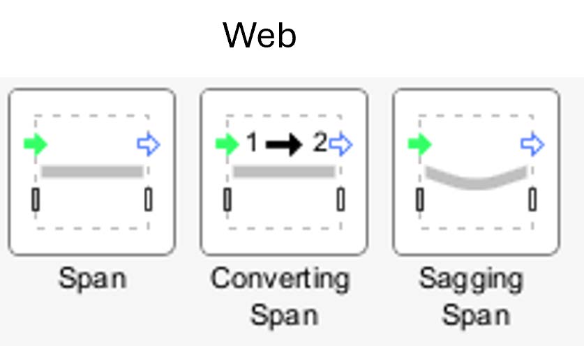
Figure 2.2: Web spans
Span - This component is used to represent the viscoelastic behavior of the web material as it moves through the system.
Converting Span - This component is used to represent a transition zone where the web material properties change from one type to another.
Sagging Span - This component is used to simulate the influence of gravity on the web span. It captures the sagging behavior that occurs when the web hangs between two rollers under its own weight.
Rollers are essential components that guide and support the web material as it travels through the system, playing a crucial role in roll-to-roll (R2R) processes. The Web Handling Library offers a comprehensive selection of roller components, enabling users to accurately model the mechanical behavior and dynamics of their systems. This section includes;
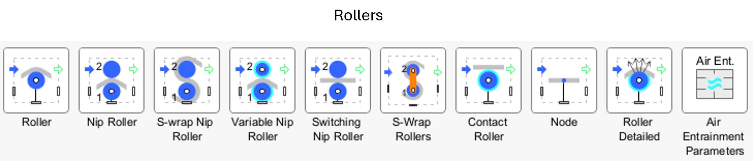
Figure 2.3: Rollers
Roller - The Roller component is used to represent either a pull roller or an idler roller within the system.
Nip Roller - This component is designed to capture the interaction between a pair of rollers, more specifically a nip roller and a companion rollers. The key distinction of this component from a regular roller is the inclusion of additional dynamics—specifically, the combined inertia and bearing friction from both rollers in the pair. This added complexity allows for a more accurate representation of systems where the interaction between two rotating bodies influences the web’s motion and tension characteristics.
S-wrap Nip Roller - This component simulates a pair of rollers—a nip and a roller—through which the web is guided, wrapping around and passing between them in an S-shaped path
Variable Nip Roller - This component is designed to simulate a system consisting of two rollers: one represents the nip, where the material is pressed between the rollers, and the other functions as the roller that interacts with the nip.
Switching Nip Roller - This component is designed to simulate a pair of interacting rollers—specifically, a nip and a companion roller. While it shares similarities with the standard Nip Roller component in its basic structure, it introduces a key functional difference: the ability to dynamically switch the upstream and downstream web spans between the two rollers over the course of the simulation.
S-wrap Roller - The S-Wrap Rollers component simulates a pair of pull rollers arranged in an S-Wrap configuration, where the web material follows an S-shaped path as it wraps around the rollers.
Contact Roller - The Contact Roller component represents a single roller that has the ability to either engage with or disengage from the web during operation.
Node - This component simulates an ideal roller with zero radius. It represents an idealized point that enables interaction with or manipulation of the web from one side to the other without affecting dimensions, sizes, wrap angles, or other geometric properties. It is particularly useful for simplified, abstract analyses.
Roller Detailed - Slippage within a model can significantly impact the performance of a roll-to-roll (R2R) system. This component represents a pull roller that incorporates the effects of slippage between the roller surface and the web
Air Entrainment - This component stores the parameters that define the impact of air entrainment on a roller.
This section contains the components that define the boundary conditions of a roll-to-roll (R2R) model. In many cases, it is not necessary to model the entire system, but instead, it is more efficient to focus on a specific portion of the web line that is of particular interest. This approach can significantly reduce modeling time and complexity. The components in this section provide the means to set the boundaries for such a model, enabling the user to define the limits of the system being analyzed while maintaining the accuracy of the simulation for the selected region.
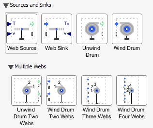
Figure 2.4: Sources and Sinks
Web Source - This component models an ideal web source with either a Speed and Tension input or by just specifying Tension alone.
Web Sink - This component represents an ideal web sink placed at the end of the web line. Here you can specify either a speed or tension as an input.
Unwind Drum - This component simulates an unwind drum featuring a variable roll radius and inertia used to model the dynamics of a drum as it unwinds the material from the roll.
Wind Drum - - This component simulates an wind drum featuring a variable roll radius and inertia used to model the dynamics of a drum as it winds the material into the roll.
Multiple Webs
Unwind Drum Two Webs - The Unwind Drum Two Webs component simulates the simultaneous unwinding of two webs, each with a variable roll radius and inertia.
Wind Drum Two Webs - The Wind Drum Two Webs component simulates the simultaneous winding of two separate webs, each featuring a variable roll radius and inertia.
Wind Drum Three Webs - The Wind Drum Three Webs component simulates the simultaneous winding of three separate webs, each with its own variable roll radius and inertia, on a single set of drums.
Wind Drum Four Webs - The Wind Drum Three Webs component simulates the simultaneous winding of four separate webs, each with its own variable roll radius and inertia, on a single set of drums.
This section contains the components that allows to model the laminatin process of R2R systems. This section contains the following components required to be used when a system contains multiple merging webs.
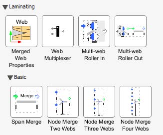
Figure 2.5: Laminating
Merged Web Properties - This property block defines the parmetes of the merged web defining the mechanics of the web and its visualization. The user can specify the web property to merge and Maplesim uses law of mixtures to determine the merged web property.
Web Multiplexer - This is purely an model organizational component used between multiple Web Roller in Component and Multi-Web Roller Out component.
Multi-Web Roller In - This component defines the entry configuration of the merging webs into the laminating rollers.
Multi-Web Roller Out - This component captures the merging of multiple webs and the exit configuration for the merged web.
Basic
Span Merge - The Span Merge component captures the merging of multiple webs from a Node Webs Merge component and the exit configuration for the merged web.
Node Merge Two Webs
Node Merge Three Webs
Node Merge Four Webs
This component can be used to divide the upstream web into two or more webs downstream. Ideally this component must be between the upstream Span and multiple downstream slitted span components forthe model to work.
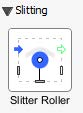
Figure 2.6: Slitting
The option for the slitting process can be found in the components property section which allows the user to specify the number of slits respectively.
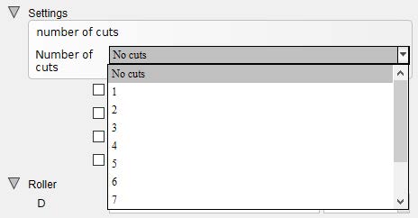
Figure 2.7: Slitting process definition
Sensors play a crucial role in extracting variable data from the simulation, which can be utilized for a variety of purposes such as control feedback, monitoring system performance etc.
Load cell - The Load Cell component measures the force components in the X and Y directions.
Inclinometer - Measure the inclination angle of the line from one frame to another.
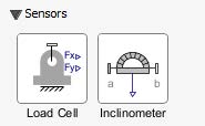
Figure 2.8: Sensors
The Primitives section of the library is a specialized subset of the Multibody library, designed specifically for modeling planar mechanisms within roll-to-roll (R2R) systems.
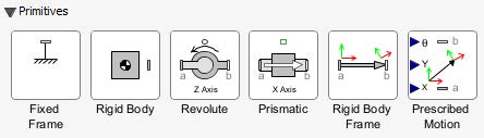
Figure 2.9: components under Primitives
Fixed Frame - A stationary frame used to position the Web handling components corresponding to the XY Plane.
Rigid Body - The Rigid Body component models a rigid body that can move in the x-y plane and rotate about the z axis.
Revolute - The Revolute component allows a rotational motion around an axis in the z-direction.
Prismatic - The Prismatic component allows translational motion along either the x or y axis.
Rigid Body Frame - The Rigid Body Frame component models a fixed displacement in the x-y plane followed by a rotation about the z-axis.
Prescribed Motion - The Prescribed Motion component converts scalar signals to translation in the X-Y plane and rotation around the Z-axis.
This section is used to simplify rouitng of the web line in a model.
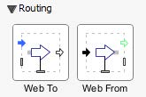
Figure 2.10: Routing Components
Web To - This component defines where the web is coming from and must be connected with the Web From component.
Web From - This component defines where the web is coming from and must be connected with the Web To component.
In this chapter, we will begin by learning how to construct a basic web handling model i.e. a simple web line. The objective is to introduce you to the foundational components and modeling techniques involved in simulating roll-to-roll (R2R) systems. Through this hands-on exercise, you will gain an understanding of how to configure the system, define key parameters, and run simulations to observe the web’s mechanical behavior.
Once the simple web line is built, we will explore how to analyze the simulation results, focusing on important variables that have impact on the system. Later we will go through the preocess of expanding the model and testing a basic control loop.
This simple web line will use 1 Unwind Drum, 3 Rollers and 3 Web Spans. The first step is the creation of the model in MapleSim. Figure 2.11 shows the model structure that will be created.
Nonetheless, we suggest following the instructions below to build the model step by step. The figure below provides an overview of the model that will be built in this section:
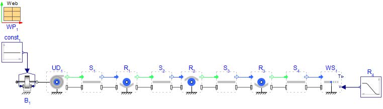
Figure 2.11: Structure of the start model
Open a new MapleSim document and save it as “StartModel.msim”.
Add a WebProperties from the Web Handling palette. The non-default parameters of the WebProperties are: W = 0.3[m], th = 0.005[m] which represent the width and thickness of the material.
Add a Unwind Drum from the Web Handling > Sources and Sinks palette. The non-default parameters of the Unwind Drum are: Dinit = 1[m], L = 0.4[m].
Check the box for Use Fixed Base within the Unwind Drum component. This allows us to define the coordinates for Drum respectively. Enter the values for the fixed base location r=[-1,0][m].
Add 4 Span components from the Web Handling > Webs palette.
Add 3 Roller components from the Web Handling > Rollers and place them between the Span components. Change the parameter L = 0.4[m], and check the box for Use Fixed Base in all Roller components.
Check the parameters of the left Roller (R1) and change the diameter D = 0.1[m]. So that, the left Roller would be smaller then the other rollers. Also in Roller R1 parameters, enter the position for the base r=[-0.3,-0.1][m].
Change the setting of the left and the right Roller (R1 and R3) and activate the "Use alternative configuration". This means the web is now under the Roller (This can be confirmed in the GUI on the canvas).
Open the parameters of Roller (R2). Change the following:
uncheck the parameter Use cylindrical geometry
mass m = 20[kg]
inertia J = 0.1[kgm].
postion for fixed base r=[0,0.5][m].
Add the fixed base position location of Roller (R3) to be r=[0.7,0][m].
Add a Web Sink from the Web Handling > Sources and Sinks palette. Check the box in the component parameters for Use Fixed Base and enter the position value r=[1,-0.1][m].
Add a Ramp block from the Signal Blocks > Common as shown in Figure 2.11. This defines the speed ramp for the startup phase of the machine. The parameters of the Ramp are:
height = 5[−]
Tr = 10[s]
Activate Smooth corners
smoothness = 0.5[−]
offset = 0[−]
T0 = 0[s]
Add a Brake2 block from the 1-D Mechanical > Rotational > Clutches and Brakes as shown in Figure 2.11. The non-default parameters of the Brake2 are: µc = 0.5[−] and reff = 0.2[m].
Add a Constant block from the Signal Blocks > Common as shown in Figure 2.11. This defines the braking force of the Brake2 . The parameter is k = 750[−].
Connect the components as shown in Figure 2.11.
Click ‘Run Simulation’ (![]() )!
)!
Once the simulation starts, The Analysis window will automatically open with the results displayed after the completion of the simulation.
At first you can see the 3D view in the 3-D Playback Window (Figure 2.12). It shows the structure of the web handling model based on the defined coordinates of the Fixed Base positions in each component and the prescribed geometry of the rollers.
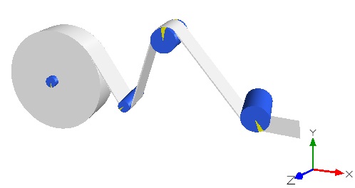
Figure 2.12: 3D view of the machine
Click on the ‘Select view type’ and change the view to ‘Front Orthographic View’. Note that the model approach is planar only and as such, the z-axis is not taken into account.
On hitting the play window we can now see the animation of the system simulated for 10 seconds time.
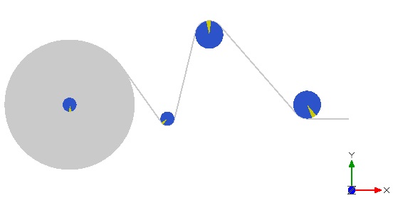
Figure 2.13: 2D depiction of the machine
Now lets gain a better understanding of the results of this model by plotting the system variables and analyzing the results. To do that lets add some probes in the canvas as shown below.
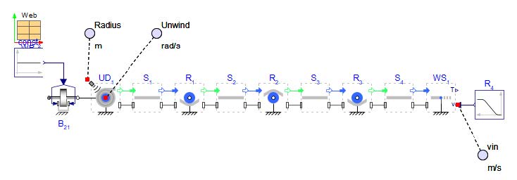
Figure 2.14: Added Probes to the Model use in Figure 2.11
The first probe is added within Unwind Drum component. The radius of the unwinder has to be selected to enable the port by checking the Enable Radius sensor in the component parameter section.
The second probe from the left measures the angular velocity of the Unwind Drum .
The last probe(From the left) measures the velocity output from the Web Sink
Once added, Click ‘Run Simulation’ (![]() )! again and view the plots in the new results window.
)! again and view the plots in the new results window.
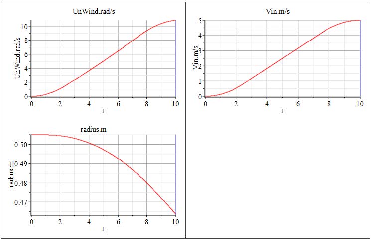
Figure 2.15: Probe plots from Start Model
These results indicate that as the radius of the Unwind Drum decreases, its angular velocity increases in proportion to the velocity specified at the Web Sink . This behavior reflects the principle of conservation of linear velocity which follows that;
v = Rω (1)
To look at the results of the Span tensions, there are multiple methods. One method is to use a probe on the component, or use the sensor that is located within the Span component. Another method is to create the tension plots in the results window. On the left-hand side palette in the results window, navigate to the section called Variables:StartModel.Latest Results, shown in Figure 2.16. Click the small icon on the far right that shows a probe symbol in square brackets - this will list all the components in the model. Presently, it only shows probed variables.
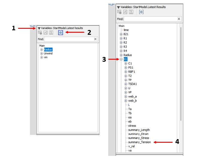
Figure 2.16: Steps to create plots from the results window
In this window there are a list of all the components in the model listed by component name. Click the plus sign (+) next to the component "S1" for Span 1 . Scrolling down there is a parameter called Summary Tension. Alternatively, if you know the name of the variable you are looking for, you can type the name of the variable in the text field Find: at the top of the window. Double click on this parameter and a new plot will open up. This plot shows the tension in Span 1 . Locate this parameter for the other 3 Span components and drag and drop them into the same plot such that they all appear on top of one another (Figure 2.17). Being able to put the parameters on the same graph allows for concise viewing and comparison.
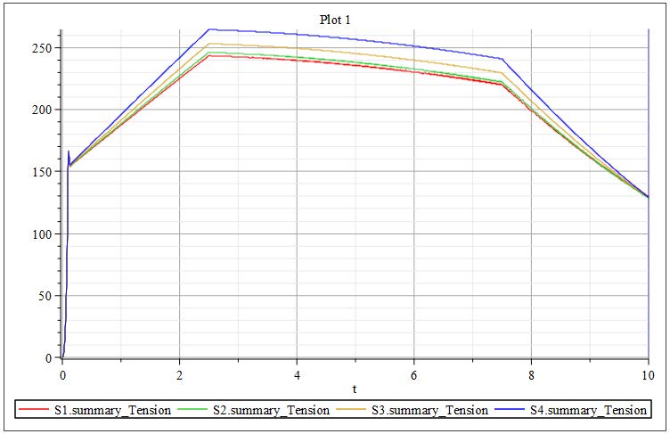
Figure 2.17: Tensions of each span in Start Model
Summary Variables are specialized output variables provided within the Web Handling Library to give users convenient access to key internal parameters in user-defined units. These variables are globally accessible throughout the library and are designed to expose important quantities such as tension, web length, wrap angle, stress, strain, web velocity, and roller angular velocity. Users can customize the units of these summary variables through the Web Property Parameter Block, allowing for consistent output formatting across the model.
This section will allow a user to understand modeling boundary conditions in a web line and how they impact the results. for this we are goinng to consider a very simple system with just one Roller, a Web Source, and a Web Sink , as well as Spans between the components (Figure 2.18). There is a constant tension input to the web line of 100[N], and a constant velocity of 1[m/s]. By manipulating the inputs of tension and velocity, it will highlight how the two are affected within web lines.
The figure below provides an overview of the model that will be built in this section:
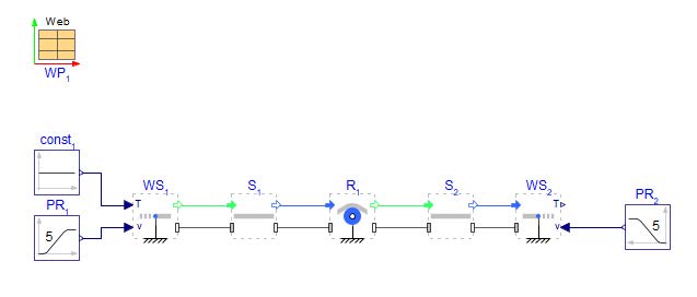
Figure 2.18: Simple model with one roller
Figure 2.19: 3D planar view of system
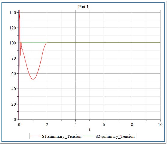
In MapleSim, a Ramp or Poly Ramp component is often used to define velocity profiles in web handling models. This approach helps prevent sudden tension spikes and ensures a smooth initialization of both speed and tension in the system. In the current example, the velocity is set to 1[m/s] at both ends of the web line, creating a consistent tension zone between the web source and sink. This is achieved by explicitly defining the downstream velocity. The results of this simulation are illustrated in Figure 2.20.
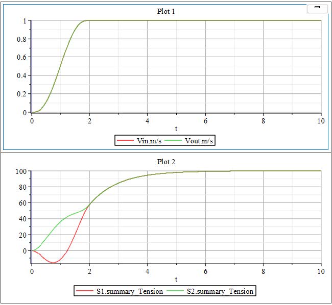
Figure 2.20: Results of simple model example
During the initial 2[s] ramp-up period, as the system velocity gradually increases, the web tension experiences noticeable fluctuations. These variations are primarily caused by the inertial effects associated with the acceleration of the Roller components. As the rollers begin to spin up from rest, their inertia resists the change in motion, resulting in dynamic tension changes within the web span.
However, once the rollers have fully accelerated and the system reaches the specified target velocity, the influence of inertia diminishes, and the system stabilizes. At this point, the tension within the web settles at a steady value of 100[N], which corresponds to the defined input tension setpoint. This steady-state condition indicates that the system has successfully transitioned through the ramp phase and achieved balanced web transport under the desired operating conditions.
There is a section of time in which the tension in Span 1 is negative, this means the web is experiencing compression. This is not possible as a web can only be in tension. How can this negative tension be addressed and ultimately reduced?
Explore - Try using larger or smaller values of velocity and tension input and see how it impacts the web line tensions and roller parameters.
The figure below provides an overview of the model that will be built in this section:
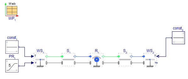
Figure 2.21: Simple model example with tension input to web sink
In this section we are going to walk through multiple methods of applying speed and tension control to a web line. The following methods will be explored in this chapter:
Applying actuation to a pull roller
Applying system data through usage of an interpolation table
Applying generated speed profile(s) in MapleSim 1D Motion Generation App
In the next section we will go a step further and apply tension zones to a web line using these methods. Figure 2.23 will be used as reference to the methods discussed.
The figure below provides an overview of the model:
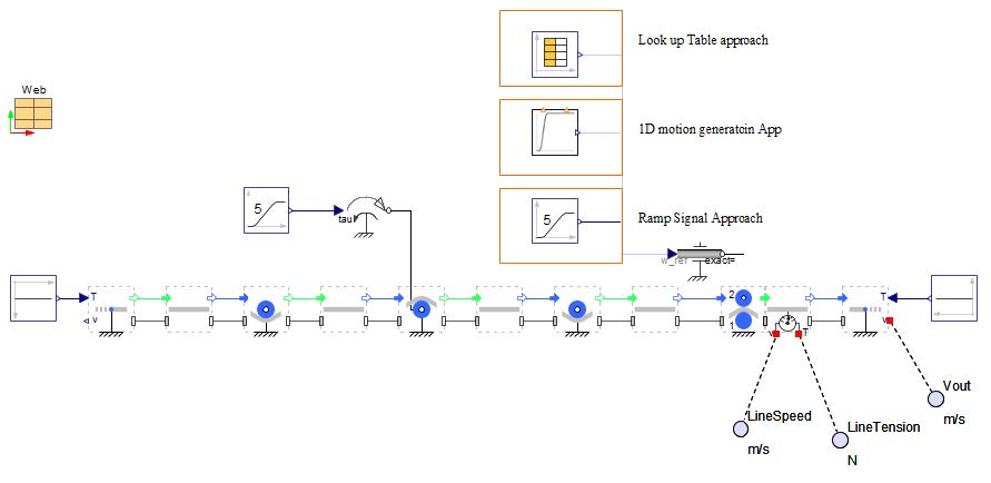
Figure 2.23: Schematic of a web line with a pull roller and actuated nip roller
Actuated Nip Roller: In the configuration illustrated in Figure 2.23, the Nip Roller is actively driven by a 1D mechanical Rotational Speed driver, which directly controls the rotational speed of the roller. This component is responsible for applying a defined speed profile to the nip roller, making it the primary drive element within the web handling system.Complementing the primary drive, a torque controller is linked to a Pull Roller , which acts as an auxiliary drive. This auxiliary roller does not dictate the web speed but contributes additional torque to assist the system.
More detailed information regarding the various Nip Rollers can be studied in the upcoming sections of the training
Pull Roller: A pull Roller is also known as a driven Roller . This is a Roller that is actuated by a motor. There are multiple methods to implement this in MapleSim, the two straightforward methods are using a Rotational Speed driver in the 1-D Mechanical > Rotational library, or by adding a Torque driver to the Roller shown in Figure 2.23. Both of these components would connect to the 1-D rotational
flange that is located at the center of each Roller component. This actuated Roller is the auxiliary drive to the Nip Roller in this system and subsequently creates a second tension zone in the system.
Using data through interpolation tables: When data is accessible, MapleSim interpolation Time Table component is a straightforward method to apply velocity and/or tension profiles to a web line. The data can be attached to the model in the form of an excel file (.xlsx) or .csv file and referenced by the component. It is vital that the first column of data is time in [seconds] and that the simulation time set in MapleSim match the time in the table in order to obtain accurate results. Using the model in Figure 2.23, deactivate (shown in Figure 2.24) the Poly Ramp and activate the Time Table for the input to the Speed Driver .
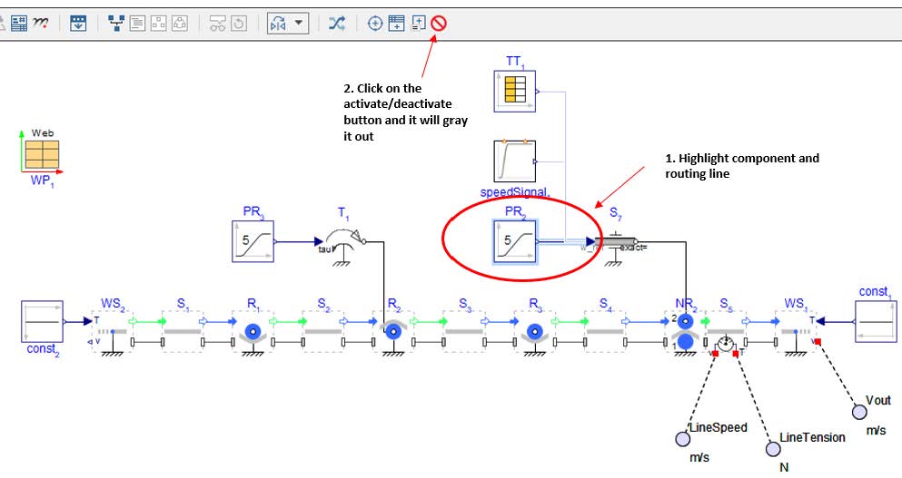
Figure 2.24: How to activate/deactivate components in MapleSim
1D Motion Generation app: The 1-D motion generation app can also be utilized to create unique curves as a signal input for the velocities of the web line. This app can be found under the Add Apps or Templates > Component Generation (Figure 2.25). Creating motion profiles in this app are explored in a separate training chapter dedicated fully to the app.
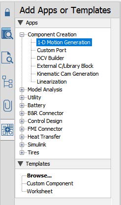
Figure 2.25: Location of 1D motion app
More detailed information on how to use the 1D motion generation App will be explained in the upcoming chapters.
Now that we’ve explored how to introduce tension and speed control into a web handling system, we can move forward by implementing tension zones within a more complex, larger-scale model. A tension zone refers to any segment of web located between two independently driven axes, such as pull rollers, actuated nip rollers, or other types of controlled rotational components.
In the previous example, we added an auxiliary drive, which effectively divided the web line into two separate tension zones. Each zone operates independently in terms of its tension profile, governed by the relative speeds of the drives at either end of the zone. If additional tension zones are required, you can simply introduce more driven or pull rollers, each configured with its own speed input. By adjusting the speed of each roller appropriately, you define the tension gradient across the web spans between them.
The tension in a Web Span arises from the difference in linear velocity between the upstream and downstream components—whether they are rollers, drums, or web sources/sinks. When one driven component rotates at a slightly higher speed than another, it stretches the web between them, creating positive tension. Conversely, if the downstream component is slower, it can reduce the tension or even introduce slack, depending on the web’s mechanical properties and material behavior.
The figure below provides an overview of the model that will be built in this section:
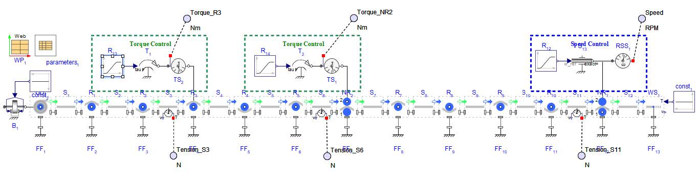
Figure 2.26: A Multi drive web line system to explore tension zones
The main drive for this example model is connected to the Nip Roller on the far right labeled NR1 . This is speed controlled and as such controls the speed of the web. It has a input of 20[rad/s] and 10[s] of ramp up.
There are two additional auxiliary drives to the system, each of which are torque controlled and thus reduce the web tension downstream. Each section of web line between the actuated rollers is a tension zone. It can be broken down into the tension zones as seen in Figure 2.27.
Zone 1 - Starts with the Unwind Drum to the first driven Roller, R3
Zone 2 - From R3 to the second actuated Roller which is a Nip Roller, NR2
Zone 3 - From NR2 to the last Nip Roller, NR1
Zone 4 - NR1 to the Web Sink (since this example ends with a truncated line, the end of the zone would be at the next location of actuation or the Wind Drum for the system).
Figure 2.27: Tension zones highlighted for multi drive example
Looking at the plotted results seen in Figure 2.28, there is a noticeable affect of each driven Roller on the web tension. The resulting simulated torques and speed of each driven Roller are stacked on top of each other along with the tensions of some Spans , allowing for ease of analysis.
Figure 2.28: Results of multi tension zone system
0 - 10 [s]: The primary drive for the line (Nip Roller 1 with Speed Driver ) is started. The velocity is increasing over the span of 10[s], reaching the target speed of 20[rad/s]. During this span of time, the web line is initializing and accelerating. There are small spikes in the tensions as the web overcomes the Roller inertias during the acceleration.
T = τ/R (2)
20 - 35 [s]: At 25[s] the second auxiliary driver Nip Roller 2 is actuated applying an additional torque to the line of 2.5[Nm]. This further reduces tensions in the line and highlights the three tension zones that have been created. The line from the Unwind Drum to R3 remains constant at 100[N], then the tension decreases by 20[N] between R3 and NR2 . The last tension zone of the line has an additional decrease of 50[N] in addition to the previous decrease of 20[N] at t=20[s].
This results in a total decrease of 70[N] down to a value of 30[N] affecting the line from NR2 to the NR1 .
This example highlights the ability to control various tension zones in one web line by utilizing a few actuated Rollers and Nip Rollers . This allows for various decreases in web tension downstream.
This section explores two methods that employ an alternate way of constructing a web line. One method is by building a section of web line that goes from right to left and another is by utilizing Maple to input configuration settings for web lines.
The figure below provides an overview of the model that will be built in this section:
Figure 2.29: Web line Reverse Model Layout
Up until now each web line has been modeled moving in the direction of left to right but not all web lines are constructed in just one direction. This section will discuss how to create web lines that move from right to left and incorporate portions that also move from left to right. The model that will be built will reflect Figure 2.30. There will be an Unwind Drum that feeds into a configuration of rollers moving from left to right then the line will make a 90 degree turn and change direction to be moving from right to left into a Wind Drum.
Figure 2.30: 3D view of the web handling machine
Open a new MapleSim document and save it as “WebLineReverse.msim”. Start with the lower path first, this is similar to creating the model in the first section. Place and connect the required components like the model structure specified in Figure 2.31.
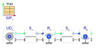
Figure 2.31: First part of the model structure
Now starts the section of web that runs in the opposite direction (right to left). A good way to model it is using the Flip Direction box within the Roller component as seen in Figure 2.32. This will place a coordinate frame at the top left corner of the Roller icon as an indication that it is flipped. This indicates that the web is now traveling from right to left (Figure 2.33).
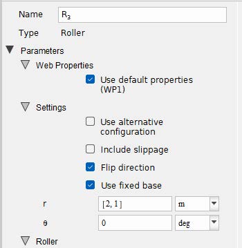
Figure 2.32: Location of Flip Direction Box in component
![]()
Figure 2.33: Roller Icon with flip direction box checked
Because of the flip direction box, the components do not have to be rotated. However, to match the direction of the line with what is on the canvas, the components can be flipped horizontally (right click and flip horizontal or CTRL + H). Doing one flip horizontal in combination with the Flip Direction box will change the web line direction from left to right to be from right to left.
Add the Span S3 and connect it with Roller R2. Optional: Rotate the span once counterclockwise.
Add the Roller R3, check the box for Flip Direction, also check the box for Use Fixed base. Connect it with Span S3. Flip the component once horizontally.
Repeat the last step with Span S4, Roller R4, Span S5, Wind Drum WD1.
Define the positions in each Roller Fixed base according to the following table:
Roller |
UD1 |
R1 |
R2 |
R3 |
R4 |
WD1 |
x [m] |
0.0 |
1.0 |
2.0 |
2.0 |
1.0 |
0.0 |
y [m] |
-0.5 |
0.0 |
0.0 |
1.0 |
1.0 |
1.5 |
Connect all components and change whether the span is on top of or under the Roller by toggling on or off the Use alternative configuration parameter for the corresponding Rollers as can be seen in Figure 2.34.
Figure 2.34 shows the model structure of the entire model.
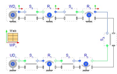
Figure 2.34: Entire model structure
Click ‘Run Simulation’ ( ![]() ) and check the 3D view! There are no probes in the model because the focus is to create the model structure. By having this option to change the direction of the web path, it provides a more intuitive and more accurate visual representation of the web line. Figure 2.35 shows how the model orientation on the MapleSim canvas now matches the 3D visualization.
) and check the 3D view! There are no probes in the model because the focus is to create the model structure. By having this option to change the direction of the web path, it provides a more intuitive and more accurate visual representation of the web line. Figure 2.35 shows how the model orientation on the MapleSim canvas now matches the 3D visualization.
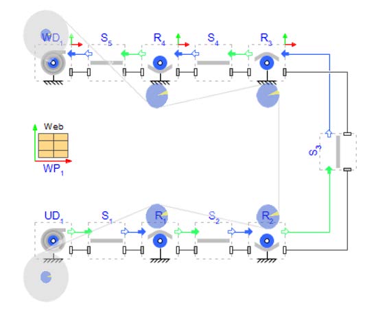
Figure 2.35: Comparing model structure and 3D view
Another example of a reverse, or right to left web path model can be found in the MapleSim example palette under Help > Examples > Web Handling Examples > Right-to-Left Web Line . See Figure 2.36.
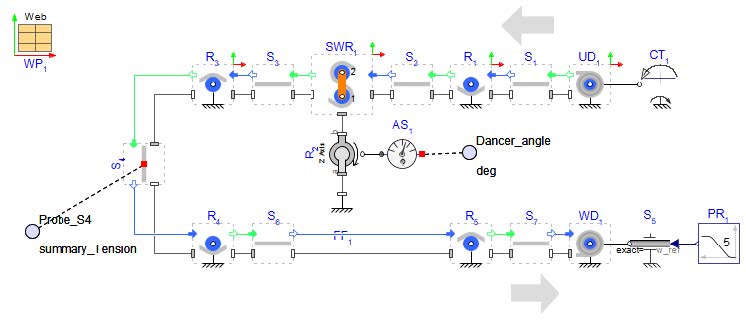
Figure 2.36: MapleSim model of a right to left orientated web line
The following sub section captures the main parts of most Web Handling simulation projects in MapleSim. The required information is broken down to three (color-coded) levels. Every next level needs the information of the level before.
Level 1 model: This is the initial model capturing the web line basics. It is useful to study the modeling capabilities and to establish a plan for adding the required detail/fidelity for validation and focused parameter/design studies in the subsequent phases.
All axes: Pull Rollers, Idle Rollers, Nips, and Wind/Unwind drums:
Axes coordinates: Essential! MapleSim assumes that the web path is in the XY plane (Z is perpendicular to the plane of the machine)
Diameters: Essential! For simple cases (or for a first-pass model), diameter, inner diameter, length, and material density can be used to calculate mass and inertia of the rollers (and wind/unwind cores).
Length: Is used in visualization.
Inner diameters: Is used in visualization.
Dancer:
Force: Essential! With applicable units.
Position: Essential!
Web properties:
Width: Essential! Is needed also for visualization.
Thickness: Essential!
Controllers: Basic information about the control structure is required. The initial model (Level 1) is created with built-in components.
Level 2 model: The added detail in this phase would be required to ensure the model can be validated against the available measurements through capturing most of the important dynamic features of the web line.
All axes: Pull Rollers, Idle Rollers, Nips, and Wind/Unwind drums:
Density: For simple cases (or for a first-pass model), diameter, inner diameter, length, and material density can be used to calculate mass and inertia of the rollers (and wind/unwind cores).
Inertia and Mass: For more complex shapes, users can choose to enter mass and inertia directly. This is not needed if cylindrical geometry is assumed. A good estimate of roller inertia is important to simulate the effects of web acceleration/deceleration on tension.
Bearing drag: In many cases, this can be ignored. It is more important for low tension usecases.
Surface coefficient of friction: If slippage is included in the model, the friction value is an essential parameter (but it may be possible to infer its value from system measurements). If slippage is not included, the friction value is only used to assess the feasibility of the calculated upstream/downstream tension ratio for each roller.
Dancer:
Mass: Required! The total mass (excluding the idler) of the moving parts of the linear dancer is needed to model the effect of acceleration/deceleration (including gravity).
Web properties:
Modulus of Elasticity: When the web is stiff and/or under low tension (i.e. When strains are very small), the overall stiffness of the spans play a small part in the simulation results (unless we are concerned with effects like resonance).
Poisson’s ratio: Similarly, the Poisson’s ratio is important when dealing with stretchy material.
Density: It is needed to calculate the correct inertia of wind/unwind drums but in general it is only a concern for heavier webs or in much more precise conditions.
Sensors:
Load cell: Required! All tensions are available in simulation. Here we just need to know where the load cells are located on the machine. It is important to include the units used in display and the units used in feedback to the controller (if different).
Encoder: Required! All roller speeds are available in simulation. Here we just need to know where the encoders are located on the machine. In simulation we can use "web speed" or "roller surface speed" if there is significant slippage. It is important to include the units used in the display and the units used in feedback to the controller (if different).
Roll radius: Roll radius is available in simulation. It can also be recalculated from speeds. Information on the actual sensor is needed to replicate the signal used in any controller for higher simulation accuracy.
Level 3 model: Detail study of the system behavior using the Level 2 model may necessitate expanding the model with additional features.
All axes: Pull Rollers, Idle Rollers, Nips, and Wind/Unwind drums:
Eccentricity: Optional! If the roller eccentricity effects are to be simulated the user must provide the value of the eccentricity.
Vacuum: Optional! Definition of pressure differences.
Dancer:
Guide friction: Optional! For higher fidelity modeling, guide friction (dry and/or viscous) is required. Of course, this is only implemented if known to be significant or inferred in the model validation phase.
Actuation mechanism: Optional! For higher fidelity modeling, information on the actuation mechanism is required. E.g., piston size, line pressure (or pneumatic circuit).
Actuators:
Motor dynamics: Optional! For higher fidelity modeling, motor dynamics can be included. The first step up would be to include a second order dynamics transfer function. If necessary, an underlying speed-controlled motor including drive train can be modeled.
Driveline: Optional! Motor inertia, Gear ratio and inertia, bearing losses can be added to the model.
Controllers: For Level 3 and beyond, detailed information would be needed. This includes controller transfer functions, controller parameters like constant gains or nonlinear gains, limit definitions etc.
Advanced:
Nonlinear web properties: Optional! Where required, MapleSim can incorporate stress-strain data and or Poisson-stress data for a nonlinear web.
Air Entrainment: Optional! Where required, MapleSim can include air entrainment. Required parameters will be discussed later.
A useful model is seldom the most complex model. Not all aspects of the system are relevant to the engineering questions being asked.
Accuracy of the predictions is not an absolute concept. Engineering questions may be answered adequately with approximate simulation results.
Model deviation from reality can be attributed to many different sources:
Intentional simplifications (e.g. neglecting material nonlinearity due to a lack of data)
Unknown physics (e.g. variation in the air pressure due to outside systems)
Physics not supported (e.g. material variation in MD/CD, misalignment)
Unknown/guessed system parameters (e.g. a guessed value for the bearing friction)
Here are some general modeling tips. This is an overview and the single points will be discussed in the following training chapters.
Elasticity: Start with a linear (constant) Elastic Modulus.
Material damping: Use the default material damping. Adjust as needed. In the most cases the default value is never changed.
Density: An exact value is rarely important. Example cases are modeling slack and high acceleration/deceleration motions.
Averaged values (in all directions) should be used. Non-uniformity is not modeled.
Slippage is often an issue for real machines and must be considered in simulations. But there are different levels of detail which increases the computation effort of a model. Start always from simple to more complex models. Consider all rollers in the first simulations as non-slipping rollers and check the summaryLimit result of each roller. Is there a chance of slippage? In which operations? Can it avoid with changed controller settings (e.g. start up ramps)? If not, slippage should be actively calculated with the checked feature of the considered rollers. High speed applications can be influenced from air entrainment which is the next level of detail.
Bearing losses can normally be ignored. The default setting is zero. It can play an important role for applications with low tension levels of with a lot of idle rollers. In this case it is easy to highlight all rollers and change the value for all of them in the same time.
Ideal rollers without imbalance or eccentricity are the default rollers in a model. Add disturbances if the task it to analyze the influence of such disturbances.
Default –> Stepwise winding/unwinding considers the impact of the layer change during winding or unwinding.
Default –> Eccentricity models the same effect as in rollers.
MapleSim provides the flexibility to model moving rollers in combination with other dynamic mechanical components (such as levers), to define their direction of motion collectively referred to as dancers. This enables users to design and simulate a wide range of dancer systems, including linear and rotational dancers. These dancer mechanisms can be modeled as either passive systems, driven solely by gravity or mechanical constraints, or as active systems, actuated by technologies such as pneumatics, hydraulics, or electric motors. These dancer models are particularly useful for tension control applications within roll-to-roll (R2R) processes. They can dynamically respond to changes in web tension, compensate for disturbances, and maintain stable operation during transient conditions such as machine start-up or shutdown. Through simulation, MapleSim allows users to extract a variety of critical measurements depending on the model configuration. These include:
Web tension across individual spans
Span lengths and their variation
Roller dynamics and position changes etc.
Dancers that are actuated often are actuated through pneumatics - force from a pneumatic cylinder, or torque from an electric motor. Both forms of actuation keep a desired tension on the web around the dancer roller.
In this first example we will build a simple rotational dancer in MapleSim.
The figure below provides an overview of the model that will be built in this section:
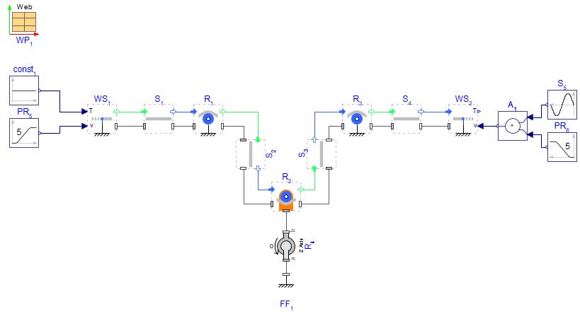
Figure 3.1: Model schematic of simple dancer
Open a new MapleSim model and save as “SimpleDancer.msim”
Add the following Web handing Library components to the canvas:
Web Properties - W =0.2[m]
1 Web Source
4 Spans
3 Rollers
1 Web Sink
in Web Handling > Primitives : 1 Fixed Frame and 1 Revolute
Add the following Signal Blocks to the canvas:
1 Constant block
2 Poly Ramp blocks
1 Sine Source block
1 Add block
Connect all the components on the canvas as can be seen in Figure 3.1 below
For the various components in the model (from right to left) fill in the corresponding parameters:
Constant - k =100
Web Source - Check Use Fixed Base use default position r =[0,0]
Check Use Fixed Base
L=0.25[m]
base position for Roller 1 : r =[0.5,0][m]
base positioin for Roller 3 : r =[0.9, 0][m]
Check Use alternative configuration
Di=0.15[m]
L=0.25[m]
Under Frame section enter frame mass mf =10[kg]
Check Add Frame Offset
For frame offset, set to rf =[-0.3,0][m]
Revolute - Change IC to be Strictly Enforce keep the IC values as default (Both 0)
Fixed Frame - position r =[1,-0.7][m]
Web Sink - Check Use Fixed Base and input position r =[1.4,0]
Sine Source - A=0.2 and T0=4[s]
Click ‘Run Simulation’ (![]() )!
)!
Figure 3.2: 3D view of a simple dancer model
By introducing a Sine Source into the web line, there are some disturbances that will affect the tension as can be seen in Figure 3.3
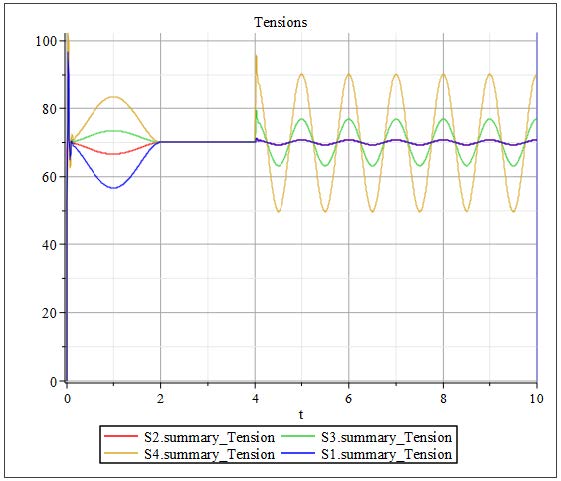
Figure 3.3: Simulation results of tensions from simple dancer model
The tension plot reveals key insights into the system’s dynamic behavior. During the first 2 seconds of the simulation, the acceleration of the web line overcomes the inertia of the rollers, resulting in noticeable fluctuations in tension across the spans. This is a typical transient response as the system adjusts to the initial motion. By the 2-second mark, the line reaches a steady velocity, and as a result, the tensions in each Span stabilize, converging to a nearly constant value of approximately 70 [N].
At 4 seconds, a disturbance is introduced in the downstream velocity, which significantly impacts the tensions, particularly in Spans 3 and 4. The dancer, which is free to rotate about its pivot point, plays a crucial role in mitigating these effects. Its ability to pivot allows it to absorb and compensate for the tension fluctuations caused by the velocity disturbance.
Specifically, when the downstream velocity signal peaks, the web is pulled more strongly, causing an increase in tension and prompting the dancer arm to pivot upward. Conversely, during drops in velocity, the tension decreases, and the dancer arm moves downward to maintain balance. This dynamic motion helps regulate upstream tension. As a result, Spans 1 and 2 experience smaller variations in tension compared to Spans 3 and 4, highlighting the dancer’s effectiveness in buffering disturbances and maintaining tension stability on the upstream side.
An example "Web Tension Control" can be found in the MapleSim example palette under Web Handling category. This example model demonstrates feedback control for a dancer arm.
Figure 3.4: Location of example in MapleSim
The model shown in Figure 3.5 incorporates a controller that uses feedback from the dancer arm angle, combined with a predefined tension input, to regulate the torque applied to the unwind drum. Additionally, the revolute joint in this example is configured with specified torsional stiffness and damping, as well as angle compensation to account for the weight of the dancer arm.
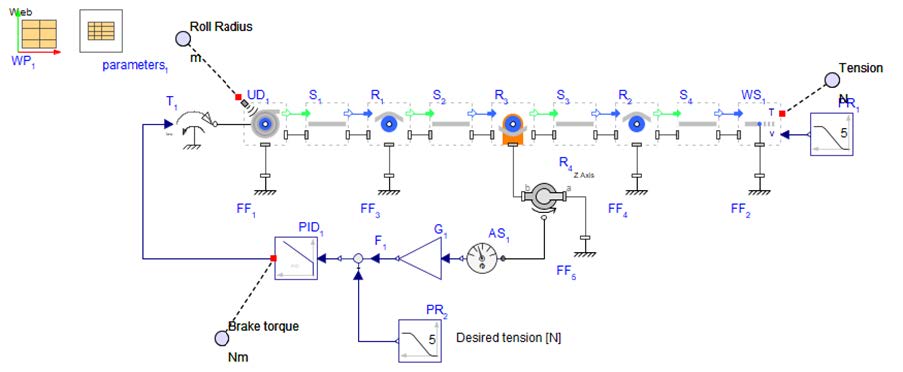
Figure 3.5: Tension Control model schematic
The simulation results shown in Figure 3.6 illustrate the system maintaining a target tension of 200 [N]. The braking torque is regulated by a PID controller, using the dancer arm angle as feedback to keep the web tension at the desired level. The output tension exhibits minor fluctuations around the 200 [N] target, reflecting the dancer arm’s continuous adjustment to stabilize the unwind web tension.
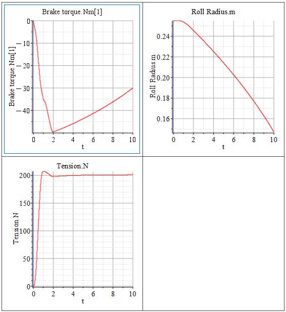
Figure 3.6: Simulated results from Tension Control dancer model
A rotational dancer is made up of two connected, movable rollers that pivot around a central point. In MapleSim, this is modeled using a Revolute joint from the Web Handling > Primitives , connected to a Fixed Frame , allowing rotation around the center point between the two Rollers that form the S-Wrap Roller .
The figure below provides an overview of the model that will be built in this section:
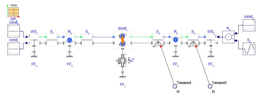
Figure 3.7: Structure of a rotational dancer model
The Web Sink uses either speed input or tension input signal, for this model the Web Sink will use the Tension input mode. There is a constant tension of 100[N] with an additional sine source disturbance.
This disturbance is activated after 3[s].
This model is using a feature of the WebHandling library that assigns color to the web based on a minimum and maximum tension value. The option (Use tension) can be selected in the WebProperties component under the section Visualization . The user can define a color and a value for the minimum and maximum limit - in this example Green (80[N]) and Red (120[N]).
Now, Click ‘Run Simulation’ (![]() )!
)!
First look at the 3D Animation view Figure 3.8. Based on the disturbance, the color of the web changes.
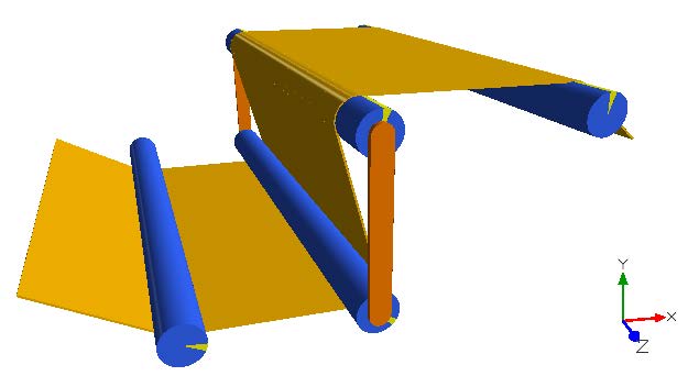
Figure 3.8: 3D view with coloring of the web spans
The model includes two probes (Figure 3.7) that measure the tension in Spans 4 and 5. Additionally, the tension within the Span located between the two rollers of the S-Wrap Roller is captured and displayed in the results window. Figure 3.9 presents the tension results for each span, labeled as Tension4.N, Tension5.N, and SWR1.weba.T . After the initial startup phase, the tension remains steady until 3 [s], when a disturbance is introduced—resulting in visible sinusoidal fluctuations across all three tension signals.
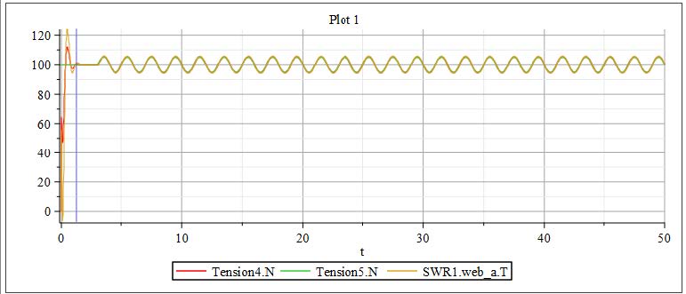
Figure 3.9: Tension diagram
Now we will control the dancer and reduce the disturbance in the Span 4 by implementing a control in the model.
However, we strongly encourage to go through the steps to built the model from scratch. The below figure shows the outline of the downloaded model. Figure 3.10 shows the model structure.
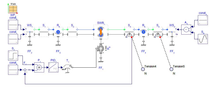
Figure 3.10: Structure of a controlled rotational dancer model
To build the above model, lets first start with the base model used in the previous section without the controller added Figure 3.7.
Add a Torque component from the 1-D Mechanical > Torque Drivers palette and connect it to the Revolute .
Add a PID controller, a Feedback , a Step and a Constant from the Signal Blocks > Common palette.
Add a Product from the Signal Blocks > Mathematical > Operators palette. Normally this is not needed but in this case it is used to activate the controller at a prescribed time. This allows for comparing the model results in the state that it was in previously to the controlled state that is being built in this model.
Change the following parameters:
Constant : k = 100[−]
Step : T0 = 20[s]
PID : k = 100[−]
PID : Ti = inf[s]
PID : Td = 0[s]
Connect the components as shown in Figure 3.10 and close the control loop.
Click ‘Run Simulation’ (![]() )!
)!
The 3D Animation (Figure 3.11) shows that the controller works well. Span 4 has nearly the same color after the controller is applied, after 20 [s].
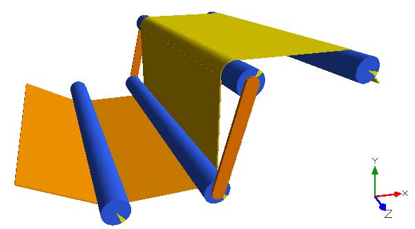
Figure 3.11: 3D view with coloring of the web spans
The curves in the diagram depicted in Figure 3.12 show the disturbance reaction starting at time 3[s] and the result of the controlled dancer at time 20[s] at which point the controller damps the tension seen in Span 4.
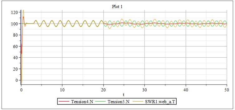
Figure 3.12: Tension diagram
Another example that is similar to the previous two examples an S-Wrap Dancer. This example is available to be explored for self-study in the MapleSim example palette under Help > Examples > Web Handling Examples > Right-to-Left Web Lines.
Figure 3.13: 3D view of S-Wrap dancer example in MapleSim
Accumulators—also known as buffers—function similarly to dancers, but their primary purpose is to store or release web material during line operation. This enables flexibility in handling varying speeds between sections of the web line, such as between the process and the winder. Unlike dancers, which primarily regulate tension, accumulators manage material flow and help maintain continuous operation. They can be either passively driven by gravity or actively driven using motors or other actuators.
MapleSim enables full customization of motion profiles, tension measurement from the accumulator’s entry to its exit, and visualization of the carriage’s movement. Additionally, you can explore the impact of bearing drag, detect potential web-to-roller slippage, and analyze other key dynamics within the accumulator system.
In the following example a simple accumulator will be built as shown in Figure 3.14.
However, we strongly encourage to go through the steps to built the model from scratch. The below figure shows the outline of the downloaded model.
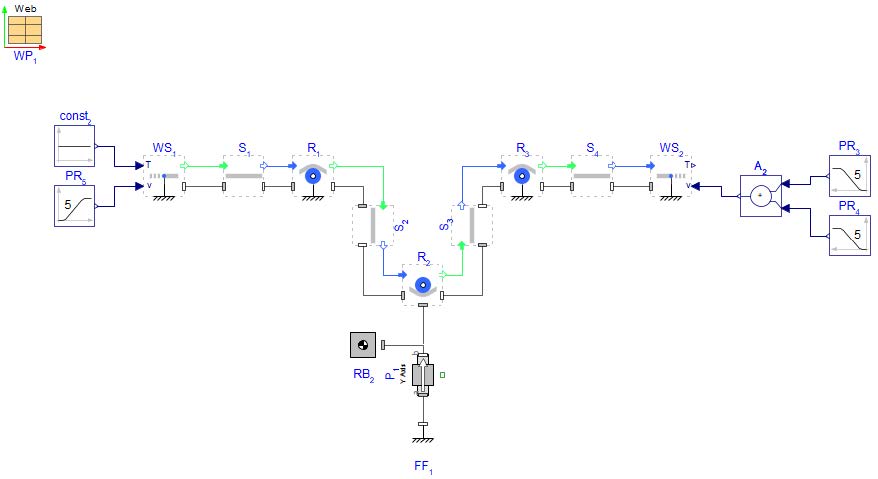
Figure 3.14: MapleSim schematic of a simple one roller accumulator.
Download a start model for this section SimpleAccumulator_start.msim
The schematic of the downloaded model is shown below. We are now going to make this model function as an accumulator.
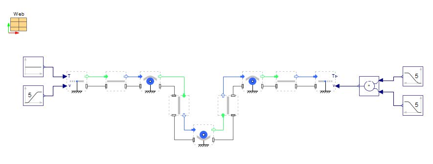
Figure 3.15: MapleSim schematic
CLick on the Roller R2 and uncheck the Use fixed base option.
Insert a Fixed Frame and Rigid Body and Prismatic. from Web Handling > Primitives and make the connections as shown in the Figure 3.14.
Change the Prismatic Axis from x-axis to y-axis.
Set the IC in the Prismatic to Strictly Enforce and keep the initial conditions at s0=0 [m] and v0=0 [m/s].
Change the Fixed Frame position to r = [0.7,-0.2]m. Connect the Fixed Frame to the Prismatic .
For Roller 2 , Set the frame mass in Roller 2 to be mf =0[kg] since this is a hanging Roller and there is no frame attached. Ensure Roller frame mass is properly accounted for when there is a hanging Roller in a system, i.e. mass=0[kg]
The signal input to Web Sink velocity needs to be updated to the following:
top Sine Source block needs to be replaced with Poly Ramp component, PR2 and update the following -
height =1.3
T0=3 [s]
bottom Poly Ramp component PR3 -
height =1.3
T0=10[s]
Click ‘Run Simulation’ (![]() )!
)!
Figure 3.16 shows the tensions in each web span . The results can be broken down into various zones based on what is happening in the system.
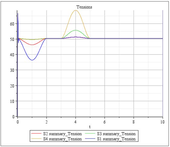
Figure 3.16: Plotted tension results of simple accumulator system
Question: How does changing the value of the mass in the Rigid Body affect the tensions of the system?
Accumulators are usually larger systems that consist of more Rollers and more elaborate frames or carriages as can be seen in Figure 3.18. There are two examples of larger accumulator systems. The first is a passive buffer.
The below figure shows the outline of the downloaded model.
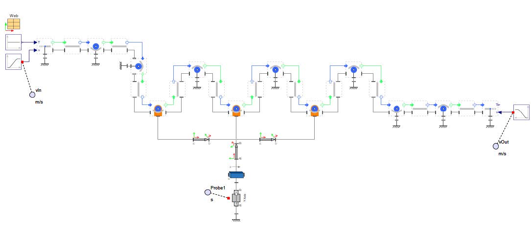
Figure 3.17: Model overview
Figure 3.18: 3-D view of passive accumulator
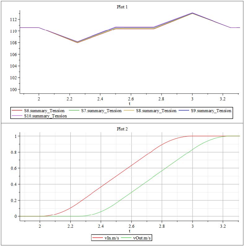
Figure 3.19: Zoomed in results of tension and velocity plots from Passive Buffer model
Figure 3.19 shows a zoomed in section of the simulation results for tension and input/output velocities. There is a noticable reaction in the Span tensions in this system to web line velocities. The acceleration at t=2[s] result in lower tensions as the velocity of the line increases. The downstream velocity is offset by 0.25[s] and once the output velocity increases at t=2.25s, the tensions in the Spans increase. The tensions increase until the velocities become constant, resulting in constant tensions.
The second example is found in MapleSim Example Palette available for self-study (the first model listed under Web Handling Examples titled “Accumulator.msim”). This is a more detailed example of a driven accumulator, as can be seen in Figure 3.20. The line has two driven Nip Rollers at either end of the accumulator that are motor driven with input/output speed profiles (created using the 1-D motion generation app). There is a detailed breakdown of the MapleSim model on the canvas for that example.
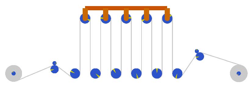
Figure 3.20: MapleSim Example of a more complex accumulator system
A few examples will be covered under the topic of web converting: Laminating - taking multiple webs and merging them into one web, Converting - the actual converting of one web to another web utilizing conservation on mass (e.g. glue is added to a cardboard web), and Discontinuous changes that has an in-going web of specific properties and an outgoing web of another property without the conservation of mass (e.g. part of the web may have been cut away).
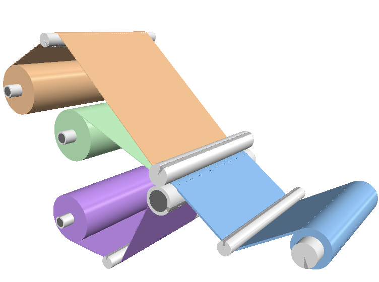
In this section the built-in MapleSim example model “Laminating.msim” is discussed to get a deeper look at the components used and its parameterization. This model contains three separate lines as input to the laminating point, shown in Figure 4.1.
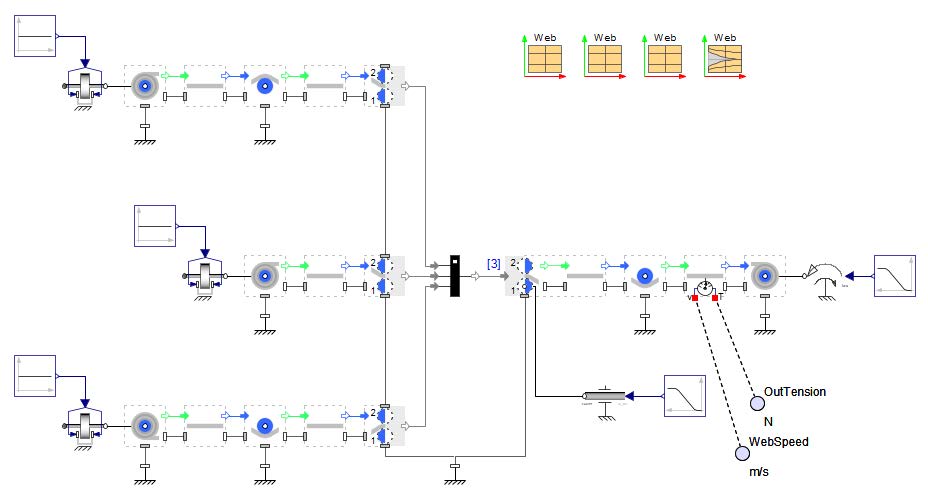
Figure 4.1: Structure of the laminating model
There are three Web Properties components to define the web properties of each line. The laminated web needs a definition of its properties as well, this is defined in the component called Merged Web Properties located in Web Handling Libaray > Laminating . This new component calculates a merged value of each parameter from the input webs. A definition of the merged webs is needed for this component, such as: MergedWebProperties = [WP1, WP2, ...]. The order in which the individual Web Properties are entered into the Merged Web Properties should correspond to the order of the actual web. The formulas for the component are written out in the associated Help page. The main formula for the parameters is written in equation (??) where x is a place holder for a parameter and i is the the i-th incoming web.
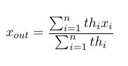
Figure 4.2: Merged Web Equation
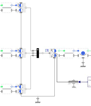
Figure 4.3: Structure of the laminating part in the model
The lamination process is modeled by several components. The last Span of each in going web line must connect with a separate Multi Web Roller In component as shown in Figure 4.3. The output signal of each Multi Web Roller In component is the input signal of the Multi Web Roller Out . This element expects a vectored input signal (see the printed [3] in Figure 4.3). A solution for that is the use of a Web Multiplexer component. The Multi Web Roller Out contains a roller pair with a span section (Figure 4.4). This component needs information about the Web Properties of the incoming and the outgoing merged web. A Roller or Web Sink component must be connected after the Multi Web Roller Out before attached to another Roller in the system.
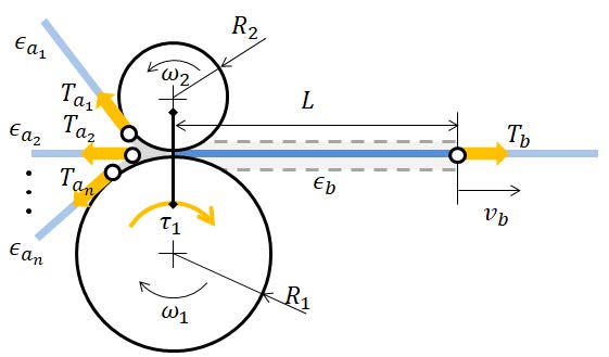
Figure 4.4: Scheme of the model approach of the Multi Web Roller Out
The Unwind Drum is connected with a rotational Brake from the 1-D Mechanical > Rotational > Clutches and Brakes package. This leads to a tension force on the outgoing web of the Unwind Drum. The Wind Drum is driven by a Torque source from the 1-D Mechanical > Rotational > Torque Drivers package. This allows for pre-tensioned of the web line within the first second of the simulation.
One of the Rollers within the Multi Web Roller Out is driven with a speed driver. The drive startup for this example model happens from 1 to 5[s] as shown in Figure 4.5.
Click ‘Run Simulation’ (![]() )!
)!
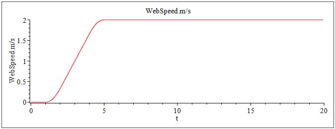
Figure 4.5: Results: Plot of the web speed
Figure 4.6 presents the curve of the strain of the in-going web lines at the lamination point. There are some observable oscillations during the startup phase. After start up time of 5 [s], the web line obtains a constant speed. The strain increases slightly over time as the radius of the Unwind Drum components decrease. On the other side (Wind Drum ), the tension in the Span (Figure 4.7) decreases after the startup phase. This decrease is due to the constant torque Wind Drum drive and the increasing radius.
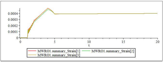
Figure 4.6: Results: Plot of the strain of the in-going web lines
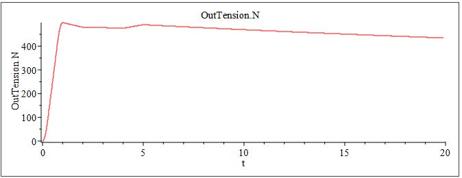
Figure 4.7: Results: Plot of the tension of the last span
Converting web is when a web undergoes a change in material properties while still conserving mass. Some examples are: calendaring (when a single material is squeezed), flutting (when a single material is ridged), or drawing (plastic deformation). The example model that will be analyzed for this section is from the MapleSim example platte called “WebConverting.msim”, open from the help menu in MapleSim. Schematic shown in Figure 4.8.
Figure 4.8: MapleSim canvas schematic of web converting example
As mentioned in the introduction to this chapter, web converting considers a web of specific properties, and then converts it to a web of new properties. As such, the model needs two Web Properties components and each Span, Roller, Wind/Unwind drum, Web Source, Web Sink etc. needs to be referenced to the correctly intended Web Properties to achieve desired results. A component called a Converting Span should be used in the location of the web line where one web property is converted to another web property. This component can be found in Web Handling Library > Webs. In Figure 4.8, there is another component used called a Node also found in Web Handling Library > Webs. The Node component models an ideal (zero radius) roller with an optional speed input (not used in this model). The Node in this example allows for a defined point in the web line and is used to set the length of the Converting Span range.
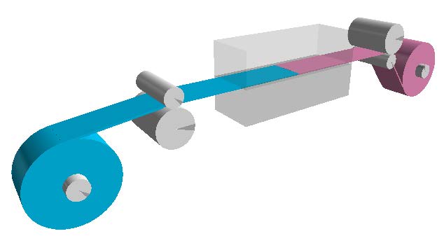
Figure 4.9: 3D visualization of converting web model
In Figure 4.9, the modulus of elasticity and the thickness of the web is changed - the web enters with web properties of WP1 in blue and exits with properties of WP2 in pink. The thickness of WP2 is half that of WP1 and the modulus E of WP2 is a quarter that of WP1.
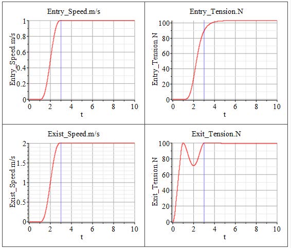
Figure 4.10: Simulation results of web converting model
This model follows the conservation of mass as part of it’s governing equations below, as such the upstream and downstream velocities have to be adjusted to obey the equations. From Figure 4.10, the exit speed is twice that of the entry speed.
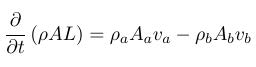
Figure 4.11: Conservation Equation
Discontinuous change is when any material is added or removed from the web without laminating, this would include processes such as drying, printing, adding glue, cutting, stamping, etc.
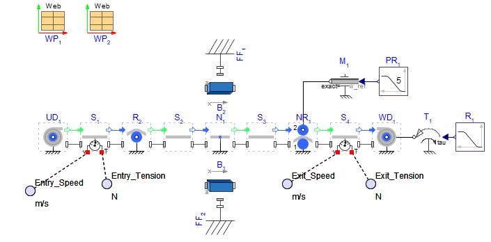
Figure 4.12: MapleSim schematic of web cutting model
In this example (Figure 4.12), a web is being cut. The width of the web is reducing from 0.2 [m] to 0.1 [m]. A few assumptions and simplifications to note: there is no actual cutting action being modeled, there is no affect from the scraps, the model does include visualization of cutting bricks (boxes shown in Figure 4.13) but it is purely visualization, and asymmetrical cutting is unable to be modeled at this time. Only the mechanical properties of mass per unit length and stiffness, due to change in width, change from one Web Property to the other.
Just like the examples above, there will need to be multiple Web Property components used for the number of changes to the web that will be occurring in the modeled section of web line. This example only changes properties once so there is only WP1 and WP2. If the width is change as it is done in this example the parameter Width option of span S3 has to be changed to Downstream.
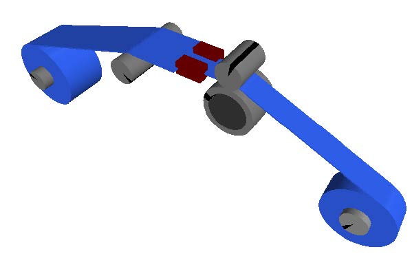
Figure 4.13: 3D visualization of web cutting model
It can be seen in the tensions seen at the entry Span 1 increases while the exit Span 4 decreases. This comes from the lack of tension control in the web line as well as the changing radius of the drums.
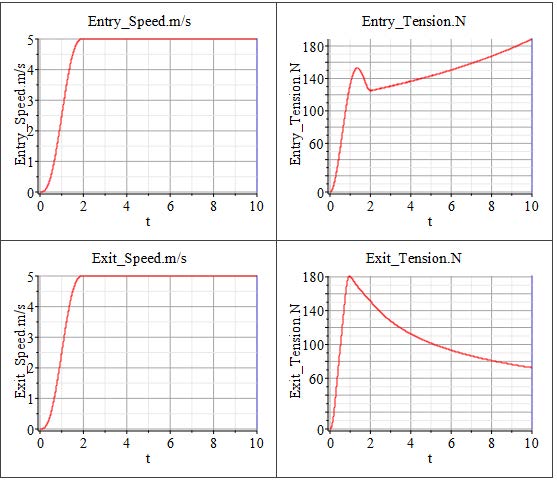
Figure 4.14: Simulation results from web cutting model
The Web Handling: Drives and Controls sub library offers a straightforward approach for defining speed profiles and implementing tension control loops in roll-to-roll processes. It allows users to efficiently organize the web line model and supports the testing and fine-tuning of control parameters in a clear and structured way.
A common method used with PLCs for tension control involves adjusting the speed of a roller or winder. In this approach, the tension controller modifies the local web speed within the web line to regulate tension levels. Feedback for the controller may come from a load cell providing direct tension measurements, or from angular or positional sensors connected to a rotational or linear dancer system.Typically, the adjustment range for the local web speed is limited to around 5–10
The Figure 5.1 illustrates a typical web line setup where the master web speed is defined by a master drive located on the nip roller. On the right side, the rewinder is regulated based on tension measurements, while the unwinder is controlled using feedback from the angular position of a dancer.
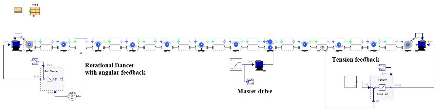
Figure 5.1: Control structure of a web line
The Drives components can also be visualized from MapleSim’s 3D viewer as well. The Figure 5.2 displays a 3D representation of the example shown above.
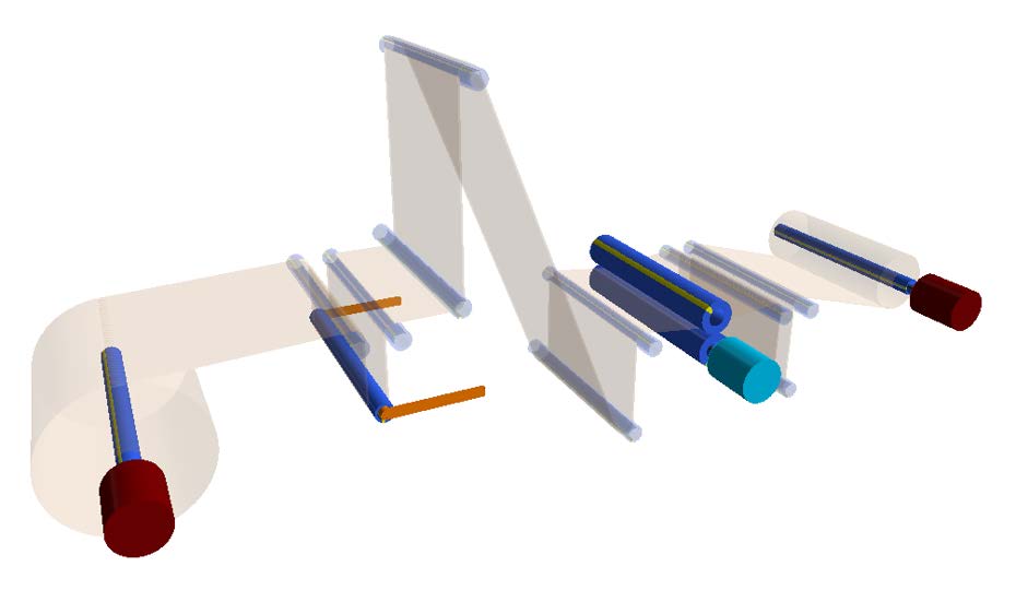
Figure 5.2: 3D view of the web line
The Web Handling: Drives and Controls sub library has two categories as shown in Figure 5.3. The Drives section includes a brake component designed to model a powder brake, along with two distinct drive implementation options. In the Controls section, users can find various components dedicated to both tension and speed control. These components offer flexibility in defining the units for each input and output signal. By default, the units are set to SI standards—torque (Nm), tension (N), radius (m), and web speed (m/s), with rotational speeds specified in revolutions per minute (rpm).
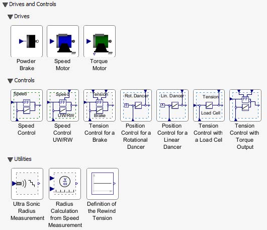
Figure 5.3: Components of the sub library Drives and Controls
All components can be visualized within the 3-D Workspace and 3-D Playback Window, allowing users to view the physical arrangement of elements within the R2R web line and to illustrate the defined tension zones. While optional, this visualization feature enhances the understanding and analysis of the R2R system layout. For accurate representation, the x-y coordinates of the motor position, as well as parameters such as roller length, motor length, and motor diameter, must be specified. Additionally, users can customize the color of components for clearer differentiation and visual clarity.
The Powder Brake component represents a simplified model of a brake system, typically used along with an Unwind Drum to generate tension in the web. This component requires a specified torque input at the tau port, which can be supplied via a reference signal or through an external control loop, such as a tension controller. The model also includes an internal inertia to represent the physical characteristics of the brake mechanism.
The Speed Motor component represents a simplified model of a motor that functions as a speed driver. It is designed to drive various elements such as Rollers (e.g., Roller, Nip Roller) or Winders (e.g., Unwind Drum, Wind Drum) based on a specified web speed. This component behaves similarly to an ideal speed-controlled motor, requiring a web speed input at the v_web port. The input can originate from a predefined reference signal or an external control system, such as a tension controller. Internally, the component computes the motor’s rotational speed using the provided web speed and the fixed radius of the connected roller. Consequently, the roller’s diameter must be specified. When connected to an Unwind Drum or Wind Drum, the radius can instead be provided dynamically through the R_act input port, allowing integration with a radius sensor or a radius estimation model. Additionally, the Speed Motor component can incorporate basic motor dynamics. When the Add simple motor dynamic option is enabled, the system includes a second-order transfer function to approximate the dynamic behavior of a real-world speed-controlled motor. In this case, the input signal is passed through a second-order filter characterized by an angular frequency and damping ratio, enabling users to simulate the motor response characteristics.
The Torque Motor component is a simplified representation of a motor that functions as a torque driver. It is designed to apply a specified torque to various components such as Rollers (e.g., Roller, Nip Roller) or Winders (e.g., Unwind Drum, Wind Drum). This component behaves similarly to an ideal torque-
controlled motor and requires a torque input at the tau port. This input can be supplied by a reference signal or generated by an external control loop, such as a speed controller .Optionally, the component allows for the modeling of a rigid driveline between the motor and the driven machine element (e.g., roller), as illustrated in Figure 5.4. It includes parameters for the motor’s rotational inertia as well as for an optional gearbox, including gear ratio settings. Motor losses can be included as speed-dependent loss allowing users to simulate its effects. Additionally, the component provides an output signal, w_meas, representing the rotational speed of the geared output shaft.
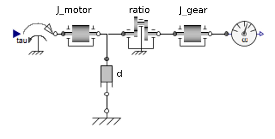
Figure 5.4: Driveline structure of the torque motor component
The Speed Motor component can be viewed as a idealized form of a speed controlled Torque Motor as shown in Figure 5.5.
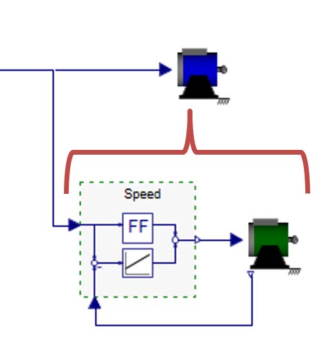
Figure 5.5: Components of the sub library Drives and Controls
The components are categorized into two groups: speed controllers and tension controllers. Each controller includes a built-in feedback mechanism implemented using the LimPID component from the SignalBlocks.Controllers library. This setup enables users to configure the PID control type, set controller parameters, and define output limits.
The tension controllers— Tension Control with a Load Cell , Position Control for a Rotational Dancer , and Position Control for a Linear Dancer — operate on the same core principle: adjusting web tension by modifying the local web speed.
The Tension Control with a Load Cell uses direct tension measurements from a load cell as the feedback signal.
The Position Control for a Rotational Dancer and Position Control for a Linear Dancer use the angular or linear position of the dancer mechanism as feedback, respectively. These components internally measure the dancer’s position and must be connected to the 1D port of the revolute (rotational) or prismatic (linear) joint in the model.
The Tension Control with Torque Output is a different approach to control tension. It is a tension controller which calculates a motor torque to control the tension of an Unwind Drum or (Re-)Wind Drum
component. This control method can be differentiated into an Indirect Tension Control and a Direct Tension control. Both approaches calculates a torque for the motor. This torque is the limit for an underlying speed controller. This controller runs with an overspeed so that the torque is always on the limit which comes from the tension control. The reason for that is a savety functionality to avoid a overturning motor in the emergency case that the web breaks. This savety feature is not needed in a simulation where a web breakage cannot be simulated. The difference between Indirect and Direct Tension Control in this case is a pure feedforward control vs. a feedforward plus feedback control of the tension as shown in Figure 5.6.
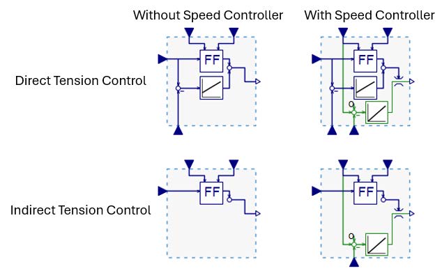
Figure 5.6: Overview of the Tension-Torque controller
The feedforward control part is a common approach for an inertia compensation of the motor, the driveline and the wound drum, a loss compensation for the bearing drag and a pre-tensioning for the reference tension.

Figure 5.7: Feedforward torque
depending of the current diameter D. "a" is the sign definition depending on the usage of the controller for a unwinder (a=-1) or an Winder (a=1). Figure 5.8 presents a an example model for a winder.
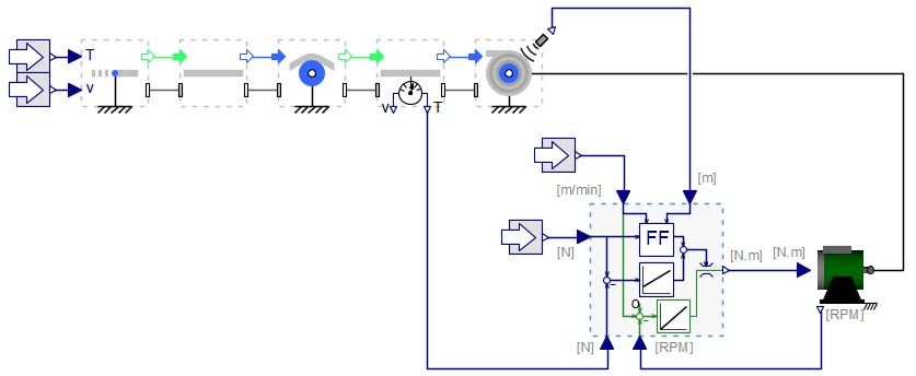
Figure 5.8: Model diagram with Tension-Torque controller
Additionally, Tension Control for a Brake component outputs a brake torque signal and can be directly linked to the Powder Brake component, as illustrated in Figure ??. This controller includes a feedforward term for compensating inertia (from both the brake and the unwind drum), along with a PID feedback loop.
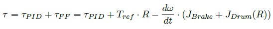
Figure 5.9: Total Torque
The Speed Control and Speed Control UW/RW components enable regulation of a specified web speed for a Torque Motor , as illustrated in Figure 5.11. Both components feature a feedforward section for inertia compensation and a feedback loop implemented with a limited PID controller. The feedforward portion uses the same parameters defined for the inertia of a roller or unwinder/rewinder, along with the web speed input, to compute the required acceleration torque.
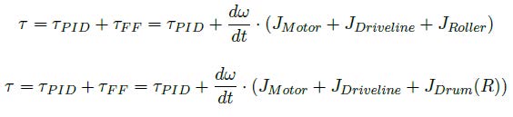
Figure 5.10: Torque for Fixed and Varying inertia
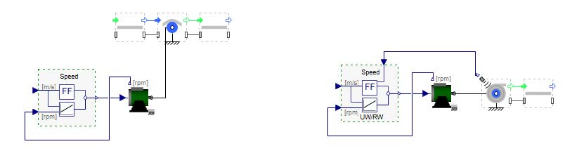
Figure 5.11: Driveline structure of the torque motor component
As the behavior of control systems becomes increasingly important, sensor effects can play a significant role. This sub library contains components to add noise on it as for real sensors are observed. The Ultra Sonic Radius Measurement component adds a quantization error to the real radius of an unwinder or a winder. Real ultrasonic sensors need a significant change of the radius to change the output value. The Radius Calculation from Speed Measurements component models a method to calculate the radius from two different speeds. The speed signal of the unwinder is needed as well as the web speed measured by an non-driven (idle) roller. There are different calculation methods for it. This component contains two approaches: (1) on sampled speed ratio and (2) on sampled position ratio (integrated speed). Figure 5.12 shows the measuring failure behavior of the components.
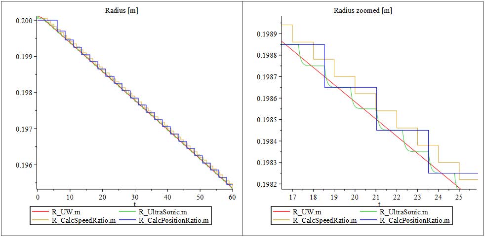
Figure 5.12: Diagrams of different radius sensor types
Another component in this sub library is the Rewind Tension Definition . The user can define a (a) constant tension, (b) a taper tension as a linear curve and (c) a nonlinear curve as a lookup table.
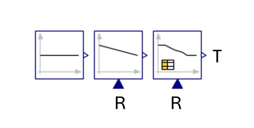
Figure 5.13: The 3 different settings for the rewind tension component
This example demonstrates the how to use Speed Motor und Tension Control with a Load Cell components to implement tension control loop for a rewinder. Figure 5.14 shows the structure of the model being developed.
However, it is advised that you go through the below steps to build the model.
The figure below provides an overview of the model that will be built in this section:
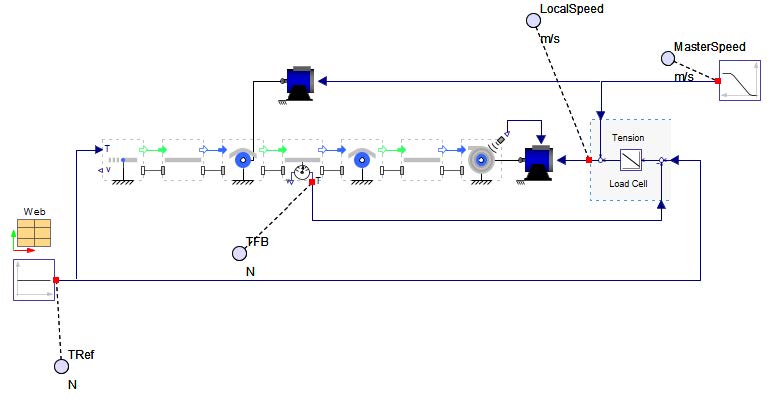
Figure 5.14: Structure of the model
Download the start model here TensionControlRewinder_StartModel.msim and save it as “TensionControlRewinder.msim”. The overview of the downloaded start model is shown below for reference.
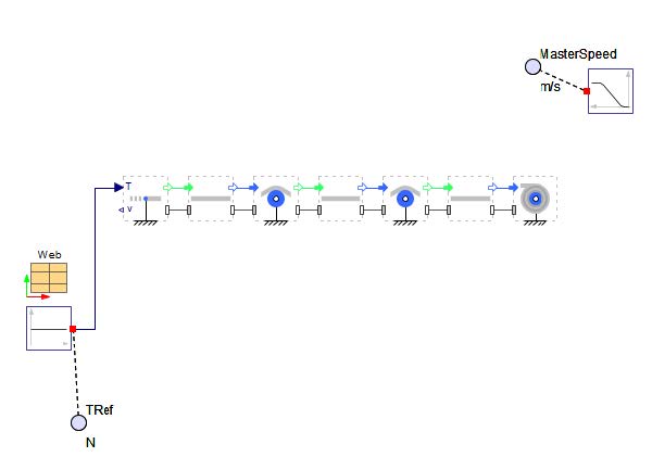
Figure 5.15: Structure of the start model
Add a Speed Motor from the Web Handling: Drives and Controls: Drives palette to serve as a master drive.
Connect it with 1D rotational port (flange_c ) of roller R1 .
Connect the signal input v_web with the ramp signal for the master speed definition.
Set the diameter D to the value from the roller R1 = 0.1[m].
Check the "Show motor" option.
Set the position r to value from the roller R1 r=[0.7,0.5][m].
Add a Speed Motor from the Web Handling: Drives and Controls: Drives palette as drive for the rewind drum.
Connect it with 1D rotational port (flange_c ) of the rewinder WD1 .
Check the "Use radius input" option.
Check the "Show motor" option.
Set the position r to value from the roller R1 r=[2.0,0.0][m].
Check the "Enable radius sensor" option of the rewinder WD1 .
Connect signal input R_max from the rewinder WD1 with R_act from the Speed Motor .
Check the "Use sensor" option of span S2 for the feedback signal of the tension control loop.
Add a Tension Control with a Load Cell from the Web Handling: Drives and Controls: Controls palette and connect it as shown in Figure 5.14.
Add probes as shown in Figure 5.14
Click ‘Run Simulation’ (![]() )!
)!
Figure 5.16 shows the simulation results. The upper plot shows the master web speed (green) and the rewinder’s local web speed (red). Zooming in the plot reveals small differences between the signals that generate the tension. The lower plot displays the reference tension (green) and the feedback signal (red).
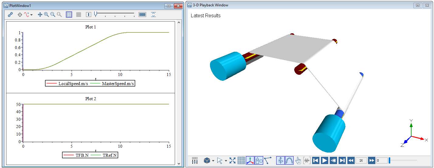
Figure 5.16: Simulation results and 3D view
Explore the settings of the tension controller. Why is it important to know and to set the order of sensor and drive?
Change the controller type of the tension controller. How does the controller type affects the control result?
Add a measurement noise to the measured radius signal. E.g. a sinusoidal signal of 0.1mm amplitude an a frequency of 100Hz. How does it affects the control result?
This example demonstrates how to use the Powder Brake und Tension Control for a Brake to create a tension control loop for an unwinder.
However, it is advised that you go through the below steps to build the model.
The figure below provides an overview of the model that will be built in this section: Figure 5.17 depicts the model structure to be created.
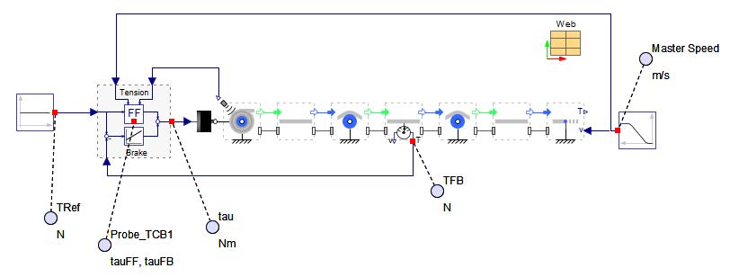
Figure 5.17: Structure of the model
Download the start model here TensionControlUnwinder_StartModel.msim and save it as “TensionControlUnwinder.msim”. The overview of the downloaded start model is shown below for reference.
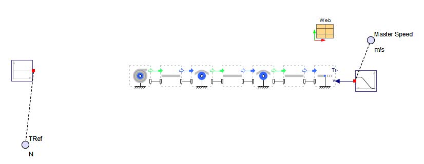
Figure 5.18: Structure of the start model
Add a Powder Brake from the Web Handling: Drives and Controls: Drives palette.
Connect it with 1D rotational port (flange_c ) of unwinder UD1 .
Check the "Show brake" option.
Set the position r to value from the unwinder UD1 r=[0,0][m].
Check the "Use sensor" option of span S2 for the feedback signal of the tension control loop.
Check the "Enable radius sensor" option of the unwinder UD1 .
Add a Tension Control with a Load Cell from the Web Handling: Drives and Controls: Controls palette and connect it as shown in Figure 5.17.
Add a Tension Control for a Brake from the Web Handling: Drives and Controls: Controls palette and connect it as shown in Figure 5.17.
Set the controller gain k to 0.2.
Set the maximal limit τmax to 1.
Set the minimal limit τmin to -1.
Add probes as shown in Figure 5.17
Click ‘Run Simulation’ (![]() )!
)!
Figure 5.19 shows the simulation results. The upper plot shows the reference tension (green) and the feedback signal (red). The lower plot shows the total braking torque (red), the feed-forward value (yellow) and the feedback value (green). It is evident that the braking torque is present at time 0s, but the tension increases at 1s when the web line starts running, indicating that the brake cannot drive the web.
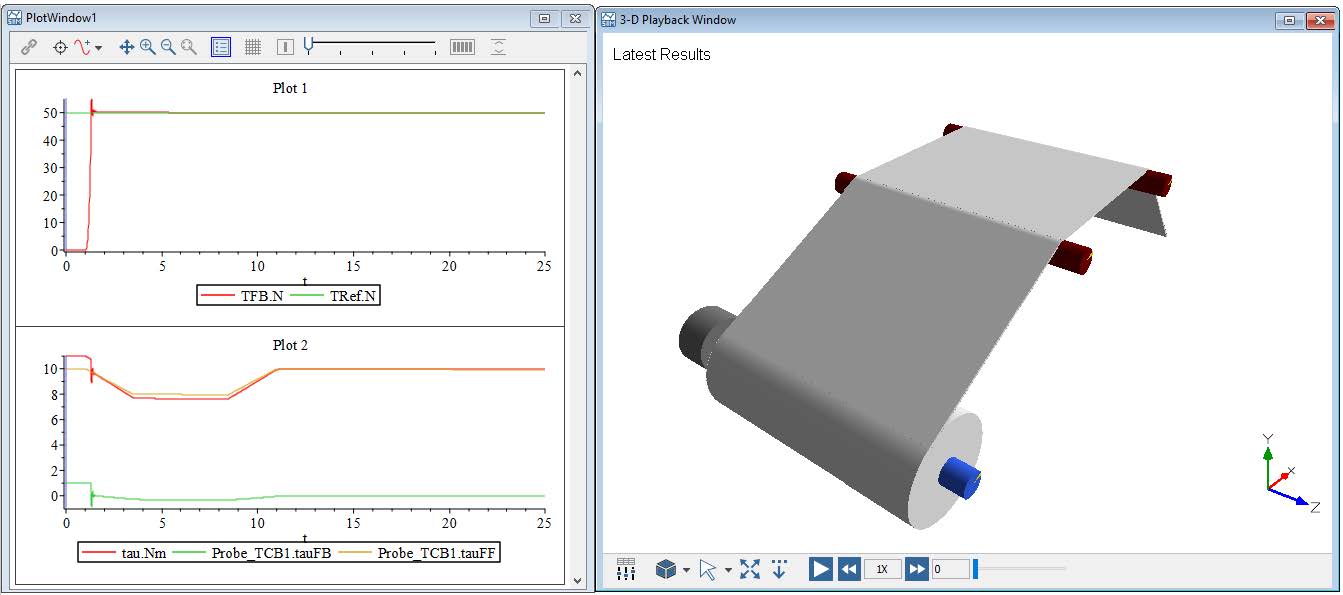
Figure 5.19: Simulation results and 3D view
What is the advantage of the feed-forward part of the tension control?
Question: How can the feedback control part be deactivated?
This example demonstrates how to use Position Control for a Rotational Dancer to create a position resp. tension control loop for an unwinder.
Download the model here TensionControlRotationalDancer.msim.
The model structure is depicted in Figure 5.20. It can be observed that the radius of the unwinder is not measured, and the only feedback for the state of the R2R process is the measured angular position of the rotational dancer.
Analyze the model structure.
Compare the defined initial diameter of the unwinder and the diameter parameter of the drive.
How is the pretension of the dancer defined?
What is the motion profile of the R2R process?
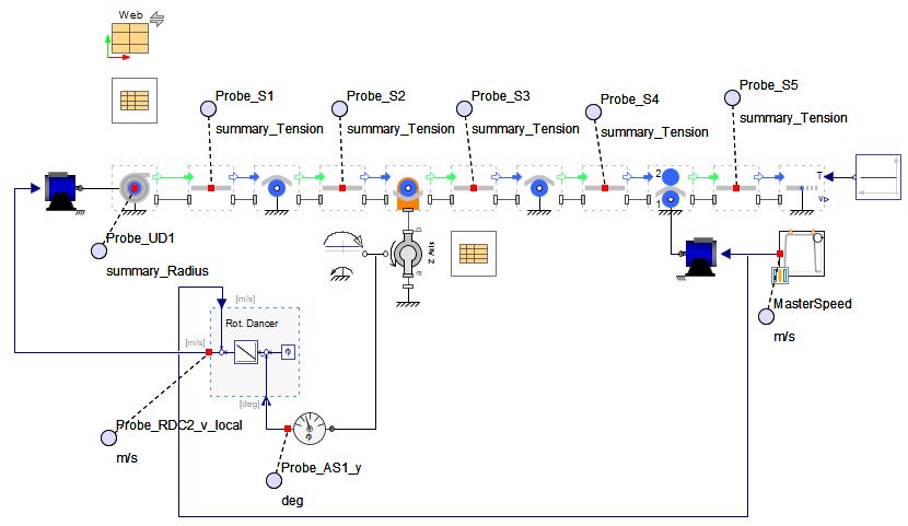
Figure 5.20: Structure of the model
Click ‘Run Simulation’ ( ![]() ). Figure 5.21 shows the simulation results and the 3Dview of the model. The upper left diagram shows the master speed (green) and the output of the controller (red). The upper right diagram displays the dancer’s angular position. The lower diagrams depict the tensions in the spans and the radius of the unwinder. It can be observed that the controller compensates for the effect of the changing radius. Larger differences between the average diameter in the unwinder drive and the current diameter of the unwinder leads to a larger movement of the dancer. The controller adjusts the local web speed for the unwinder to counteract this. This implies that the tension definition for static operations is determined by the pretension of the dancer, with the controller maintaining the dancer in the working position.
). Figure 5.21 shows the simulation results and the 3Dview of the model. The upper left diagram shows the master speed (green) and the output of the controller (red). The upper right diagram displays the dancer’s angular position. The lower diagrams depict the tensions in the spans and the radius of the unwinder. It can be observed that the controller compensates for the effect of the changing radius. Larger differences between the average diameter in the unwinder drive and the current diameter of the unwinder leads to a larger movement of the dancer. The controller adjusts the local web speed for the unwinder to counteract this. This implies that the tension definition for static operations is determined by the pretension of the dancer, with the controller maintaining the dancer in the working position.
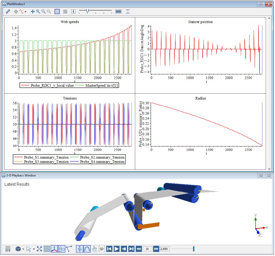
Figure 5.21: Simulation results and 3Dview
Questions
Why are there two settings in the controller?
What is the reason of the tension spikes in span S1 and S4?
This example demonstrates thow to use Position Control for a Linear Dancer to create a position resp. tension control loop for an unwinder.
Download the model here TensionControlLinearDancer.msim. The model structure is depicted in Figure 5.22. In this case the radius measurement is modeled with a sensor failure where the ultra sonic sensor signal shows a quantization error. This signal is then filtered using a first order filter.
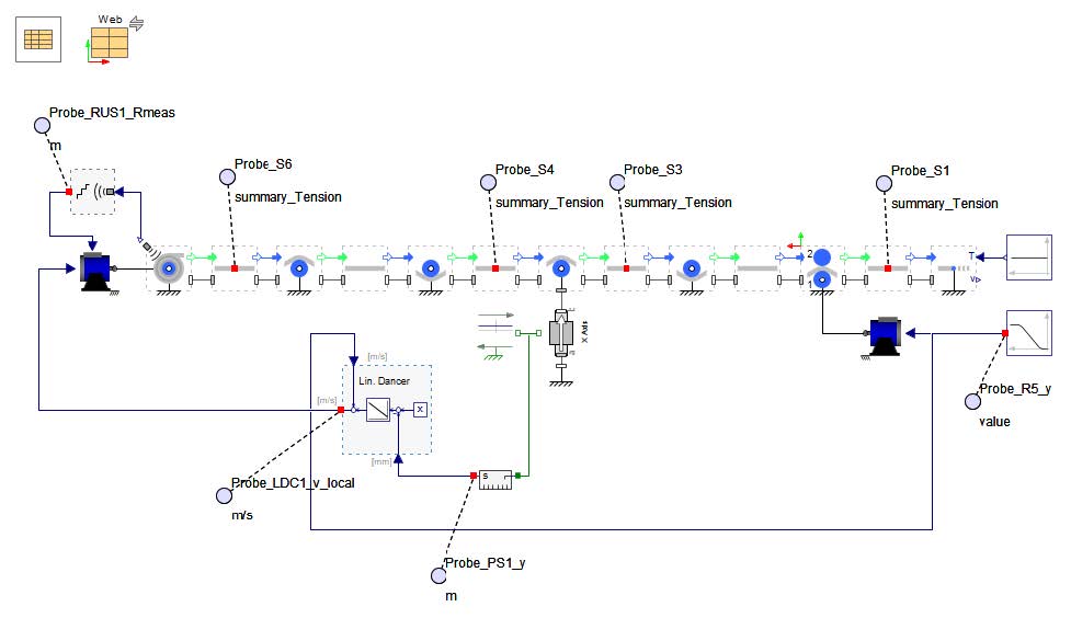
Figure 5.22: Structure of the model
Analyze the model structure.
Check the ultra sonic sensor settings.
How is the dancer pretension defined?
Click ‘Run Simulation’ ( ![]() ). Figure 5.23 shows the simulation results and the 3Dview of the model. The upper left diagram shows the master speed (green) and the output of the controller (red). The upper right diagram displays the dancer position. The lower diagrams depict the tensions in the spans and the current radius (red) and the measured radius (green) of the unwinder.
). Figure 5.23 shows the simulation results and the 3Dview of the model. The upper left diagram shows the master speed (green) and the output of the controller (red). The upper right diagram displays the dancer position. The lower diagrams depict the tensions in the spans and the current radius (red) and the measured radius (green) of the unwinder.
Explore: Decrease the controller gain k and explore what happens.
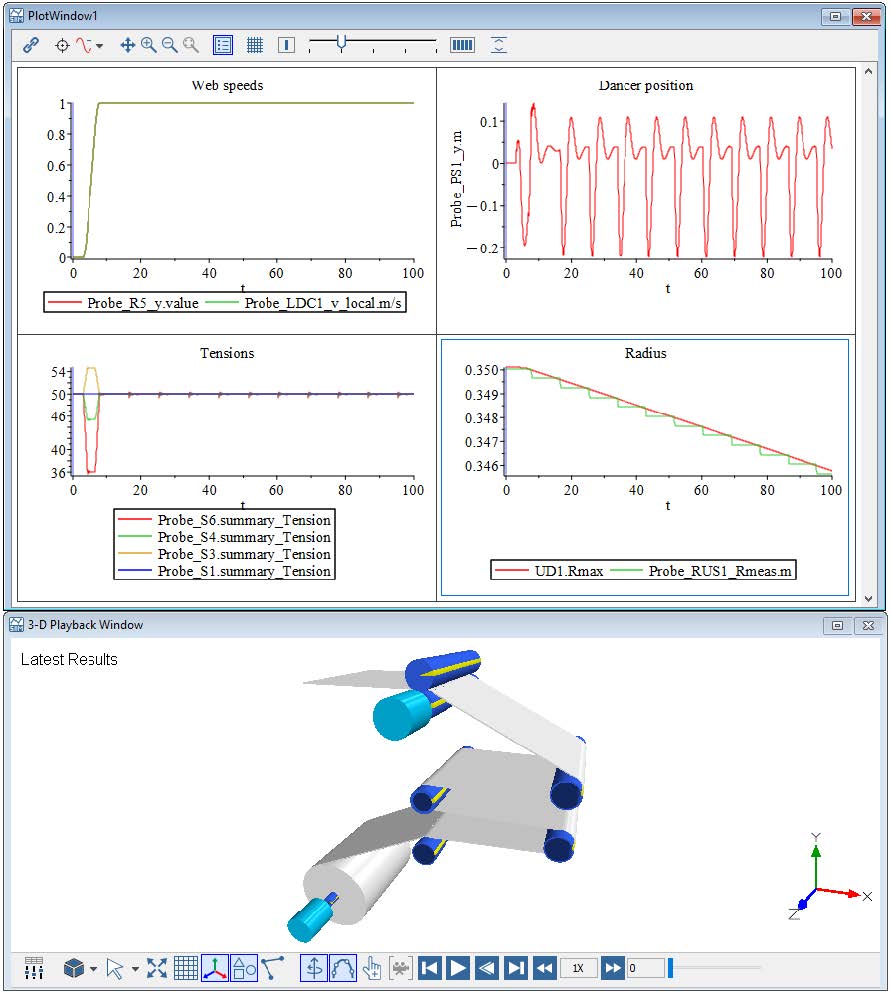
Figure 5.23: Simulation results and 3Dview
The first example demonstrated the use of a Speed Motor as as ideally speed-controlled motor and the impact of the diameter measurement on a rewinder. If it’s necessary to examine the influence of the speed controller itself, the Speed Motor can be replaced with a Torque Motor and a Speed Controller .
However, it is advised that you go through the below steps to build the model.
The figure below provides an overview of the model that will be built in this section:
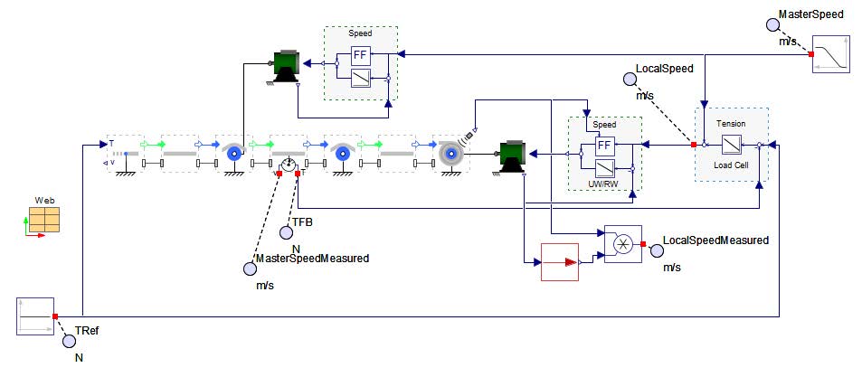
Figure 5.24: Structure of the model
Open the model completed in section 1 5.2 “TensionControlRewinder.msim” and save it as “TensionControlRewinderTorqueMotor.msim”.
Delete both Speed Motor components.
Add a Torque Motor from the Web Handling: Drives and Controls: Drives palette as master drive.
Add a Speed Controller from the Web Handling: Drives and Controls: Controls palette for the master drive and connect it as shown in Figure 5.24.
Add a Torque Motor from the Web Handling: Drives and Controls: Drives palette as rewinder drive.
Add a Speed Controller from the Web Handling: Drives and Controls: Controls palette for the rewinder drive and connect it as shown in Figure 5.24.
Add the calculation of the local web speed for the rewinder and the probes as shown in Figure 5.24.
Click ‘Run Simulation’ (![]() )!
)!
Explore: How does the control parameter of the speed controller of the rewinder influence the tension control? Change the gain k to 0.1.
This example presents the usage of the Tension Control with Torque Output . Open the model “Help: Examples/WebHandlingExamples/DrivesAndControls/TensionControlTorqueAdaptionReWinder.msim” from the examples. It presents the usage of the different modes of the component. It is possible to choose between the Indirect Tension Control mode and the Direct Tension Control mode which includes a feedback controller. The underlying speed controller is optional. In real a speed controller is needed to avoid an over-speeding of the motor in an emergency case. This is not possible in simulations but a speed controller can be activated also.
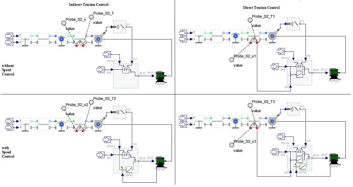
Figure 5.25: Structure of the model
Explore: What is the main difference between Indirect and Direct Tension Control?
Some common issues that are seen in web handling consist of the following: web slippage, bearing drag, and roller eccentricity.
The default setting of each Roller is a no slipping behavior, however there is the option to activate slippage when it is needed. Be aware that the activation of slippage leads to a higher computation effort and as such the solver in MapleSim will need to be changed from the default CK45 (semi-stiff) to Rosenbrock (stiff). Each Roller has a variable that can be plotted with simulation to give information regarding if the Roller is slipping or not. The variable summary_Limit shows if the tension limit is less than the capstan limit (summary_Limit=0) or reaches the capstan limit (summary_Limit=1). Once the Roller reaches a capstan limit of 1, it is safe to assume the Roller is experiencing a slip condition. Another useful variable that can be plotted for each Roller is the wrap angle of the web around the roller - (summary_WrapAngle).
However, it is advised that you go through the below steps to build the model.
The figure below provides an overview of the model that will be built in this section:
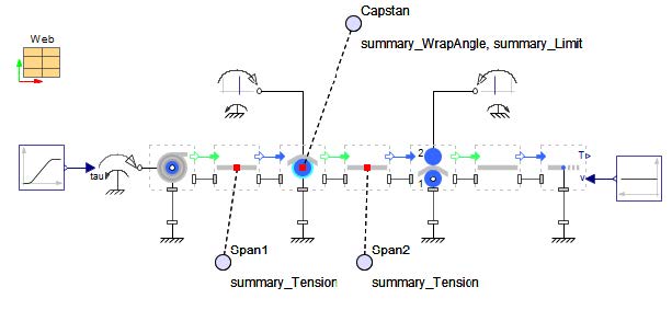
Figure 6.1: Structure of the model
Download the start model here ModelSlippage_StartModel.msim. The overview of the downloaded start model is shown below for reference Figure 6.2.
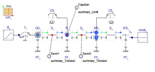
Figure 6.2: Structure of the model
Click ‘Run Simulation’ (![]() )!
)!
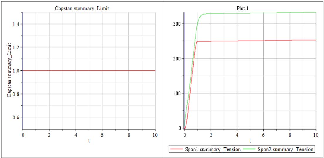
Figure 6.3: Result if slippage is not included on the roller.
Figure 6.3 shows the results of the defined probes in the model. For the duration of simulation, the summary_Limit has a value of one which indicates that the Roller, R1 is slipping under the web span for the whole simulation. It is also important to notice the plot of tension. From this plot the tension in Span 2 is roughly 100 N larger than the tension in Span 1 . From the following equation
Figure 6.4: Equation
Where µ is the coefficient of friction between the web and Roller , β is the wrap angle of the web on the Roller in [rad] and Ta and Tb are the low and high tensions on either side of a Roller , respectively. Since µ is known from the model as 0.2 and the wrap angle can be estimated approximately at 22.75[deg] (about 0.4[rad]), a quick calculation would show the ratio of Ta to Tb should be roughly 1.083. In other words, the tension in Span 2, if Span 1 tension is 250[N], should be approximately 270.75[N]. Of course, the plot shows that the tension in Span 2 is around 330[N]. It can be concluded that these are inaccurate results. We will try simulating with slippage activated on R1 so that we can be more confident that slippage is occurring.
Now set Include slippage in Roller R1. The Icon of the Roller will change as shown in Figure 6.5 with a light blue halo around the roller GUI.
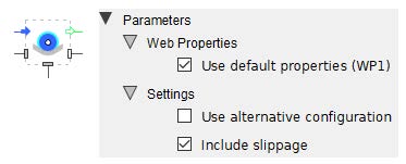
Figure 6.5: Icon and setting of a roller which includes slippage
Set the initial condition of vrel in Span 2 such that vrel=0[m/s]. Click the check mark icon next to the parameter to set it to enforce.
Add the probed value of summary_WrapAngle for R1 .
NOTE: Summary variable units can be changed in the Web Properties component under the header Summary Variables, this includes the unit for summary_WrapAngle see Figure 6.6.
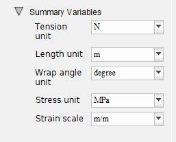
Figure 6.6: Web Properties Properties window, location of units for summary variables in a Web handling model
Change the solver to Rosenbrock
Click ‘Run Simulation’ (![]() )!
)!
With the slippage included parameter, the summary_Limit is always equal to one and does not need to be plotted. The tensions of each span are plotted again and immediately it is noticeable that there is a large change in the tension for Span 2 as shown in Figure 6.7. The tension for Span 2 has reduced drastically to approximately 270[N], as expected from the rough calculations from above. This result provides better insight into what the web line is experiencing. With slippage being included on the roller, the tension drops to more a logical and expected value. It is important to note that when slippage is included in a model, the initial conditions of the Span after the Roller with slippage should be set to enforce for vrel=0[m/s]. This is needed otherwise there will be very large spikes of tension at the beginning of the simulation. The large tension spikes are a result of the two Spans on either side of the Roller having two different initial velocities. Notice, Span 1 also has an enforced initial velocity of 0[m/s].
Figure 6.7: Result if slippage is included
Now that it is apparent the Roller is slipping, how can we remove slippage from the model all together?. There are a few things that can be adjusted to greatly reduce the chance of slippage occurring in the model.
However, it is advised that you go through the below steps to build the model.
The figure below provides an overview of the model that will be built in this section:
Figure 6.8: Structure of the model used for Slippage Prevention
The method that will be explored in this model will be changing the wrap angle on the Roller experiencing the slippage (Roller 1 ). This is done by moving the location of the adjacent Unwind Drum . Lets continue the model from the previous section and make the following changes.
Change the position of Unwind Drum from the original location of r = [-1, -0.5][m] to the new location of r = [0, -0.3][m].
Turn off the include slippage parameter so that Summary_Limit will plot again. This will show if the Roller is slipping or if this change removed slippage.
Remove the initial condition of vrel=0[m/s] that was set to enforce (check mark button) in Span 2 by clicking on the minus sign button to have MapleSim ignore the input value. If this is not completed, an error will occur during simulation.
Re-simulate the model.
Figure 6.9 shows the 3D view of the model with configuration 1 being the original orientation of the Rollers and configuration 2 being the updated orientation with the Unwind Drum moved below and closer to Roller R1 .
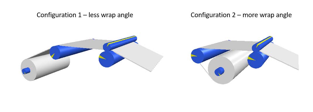
Figure 6.9: MapleSim model in two configurations.
By moving the Unwind Drum below R1, there is a larger wrap angle (as can be seen in the plots in Figure 6.10) of the web span on Roller 1 . The Summary_Limit goes to 1 at the start of simulation for a few milli-seconds as the system starts accelerating and then remains at 0 for the duration of simulation. This shows the Roller is no longer slipping.
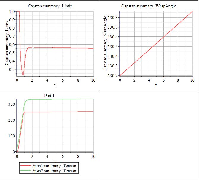
Figure 6.10: Results with larger wrap angle on Roller 1
Do you get the expected tensions in Figure 6.10 when using the equation mentioned above in this section? The friction is still 0.2 and now the new summary_WrapAngle is plotted (in degrees). If Span 1 is roughly 250[N], do you get an approximate expected tension value for Span 2 based on Figure 6.10?
As was just explored and will be explored more in the following sections, some methods of eliminating slippage include the following:
Changing the line tension or increasing the roller coefficient of friction.
Changing the wrap angle of the web on the roller - this might involve repositioning the roller or the wind/unwind drum
Add a vacuum roller to the line (this will be explored as a solution to another common issue of eccentricity in the next example)
This example, as shown in Figure 6.11 explores disturbances in the web line in the form of eccentricity and presents a method that can be used to counteract it.
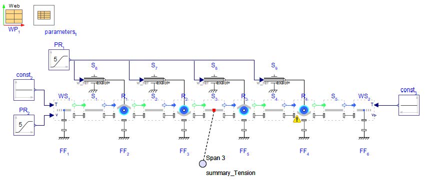
Figure 6.11: Disturbance Model Schematic
A few things to note from Figure 6.11 are the following:
Each Roller is driven, also sometimes known as pull rollers.
Each Roller has include slippage option applied - indicated by the light blue outline on the GUI for each Roller
Roller 4 has Add eccentricity option applied - indicated by the yellow warning symbol in the lower left corner of the component.
Click ‘Run Simulation’ ( ![]() ) and view the results screen. A few things can be noted about the model results right away. The probe in the model plots the tension of Span 3 . This plot (Figure 6.12) has a lot of
) and view the results screen. A few things can be noted about the model results right away. The probe in the model plots the tension of Span 3 . This plot (Figure 6.12) has a lot of
oscillation in tension after the initialization. The oscillation is from 120 to 80 [N] - roughly focused around an average tension of 100 N.
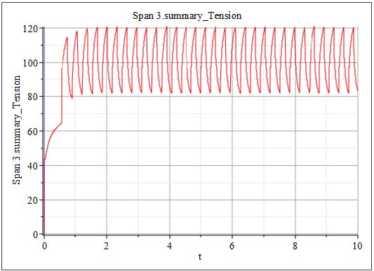
Figure 6.12: Tension results in web span 3 of Disturbance Propagation model
This tension oscillation is due to the eccentricity in Roller 4 . This issue commonly seen in web lines is due to a roller being mounted a certain distance away from the true roller center - see Figure 6.13. In this example model above, the distance that the center of rotation is away from the roller center is e = 0.001
[m] and θ0 =0[deg].
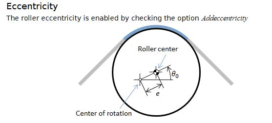
Figure 6.13: Schematic of eccentricity defined in Rollers
This issue of eccentricity can be addressed in a few ways. One way is to remount the roller as close to the roller center as possible - ideally on the actual roller center. Another method to explore through MapleSim is to add a vacuum roller to the line. In this example, Roller 3 will have vacuum added. In the parameters for Roller 3 , under Friction category, there is a location to include a surface pressure. When slippage is enabled on the roller, a positive value entered in the pressure field is considered suction surface pressure on the roller, as explained in the parameter palette (Figure 6.14).
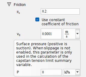
Figure 6.14: Pressure field in Roller component parameters
Enter P =30[kPa] into this field for Roller 3 and re-simulate the model. Figure 6.15 shows the updated tension in Span 3 . By introducing a vacuum roller before the roller with eccentricity, the oscillations in the span have dampen greatly.
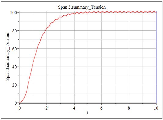
Figure 6.15: Tension results in web span 3 with vacuum applied to Roller 3
Viscous bearing drag is another common issue that is seen in web lines. Bearing drag will be added to a simple model from a previous section to analyze the affect that is seen on the tensions in a web line (Figure 6.16).
This example, as shown in Figure 6.16 explores the influence of bearing drag on the rollers.
Figure 6.16: MapleSim of two driven nip rollers
When the model is open, choose one of the provided speed signals to the Motion Driver . For example, activate the Poly Ramp and leave the Time table and 1-D Motion Generation Speed profile deactivated.
Click ‘Run Simulation’ (![]() )!
)!
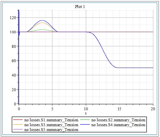
Figure 6.17: Tension results of Model
Figure 6.17 shows the tensions of the system with no losses applied to the line - the ideal tension results. The tension has an increase in the beginning as the web overcomes the Roller inertias, then settles to 100[N] until the auxiliary drive is actuated, at which point the tension reduces in Spans 3 and 4 to 50[N]
Now add bearing drag d =0.01[Nms/rad] to the Rollers R1, R2, and R3 .
Click ‘Run Simulation’ (![]() )! Look at the new tension plot.
)! Look at the new tension plot.
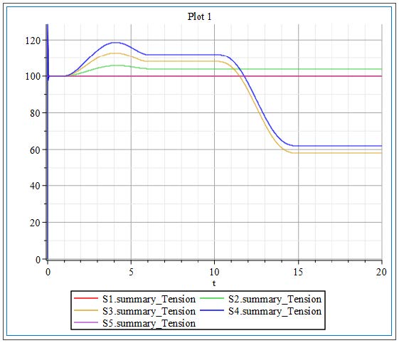
Figure 6.18: Tension results with added bearing drag
Figure 6.18 shows some increases in Span tensions in Spans 2, 3, and 4 not only during ramp up of the web line but also during the 5[s] of constant tension in the system (between t=6 [s] and t=11[s]) the Spans experience higher values. When the auxiliary drive starts, the Spans affected (Spans 3 and 4 ) reduce in tension. The added resistances of bearing drag in the Rollers result in some higher tensions, as well as the decrease in tensions after the auxiliary drive due to more material coming in than going out at that location in the line.
Change the bearing drag to higher values and see how it affects the tensions. Does high bearing drag affect any other aspects of the line?
This chapter shares ideas of modeling special effects, configurations or mechanisms of an R2R process. These ideas came across in discussions with customer about practical issues and use cases.
There are process steps where the web is moved over a plate for heating or cooling purposes. Beside the thermal behavior is the tension behavior based on the friction loss an interesting question.
How can it be modeled in MapleSim? The basic idea is to consider the heating plate as a curved plate which can be considered as a fixed roller. The principle model approach is shown in this section.
Figure 7.1 shows the model structure. There is a master drive which defines the web speed and a roller which is fixed on the 1D rotational port and uses the active slippage option. This roller models the plate over which the web moves, and the slippage models the friction loss.
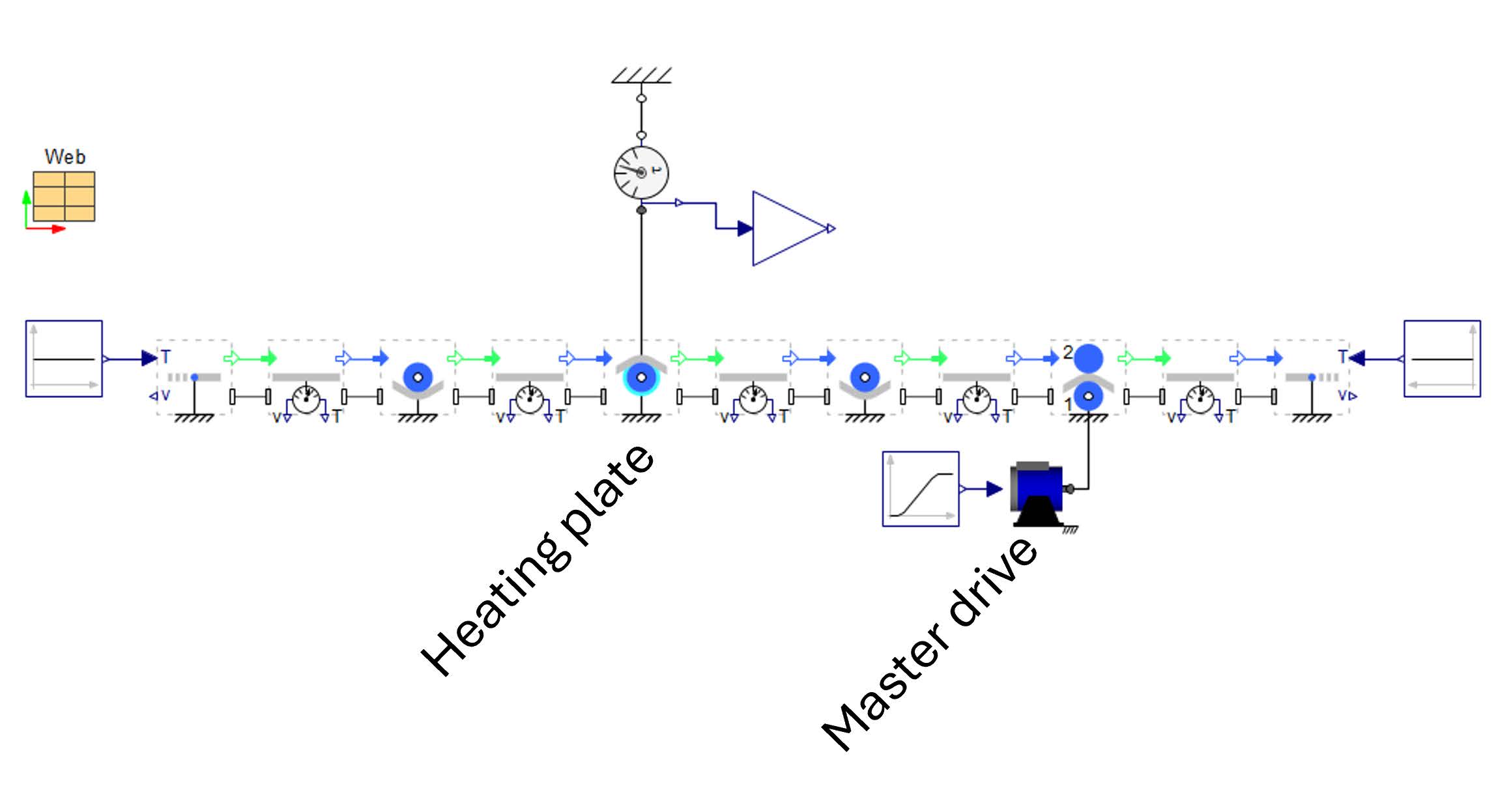
Figure 7.1: Structure of the model
Figure 7.1 shows the results. The 3D visualization uses different color for the web depending on the tension. It visualizes the different tension levels depending on the friction losses through the slippage. The diagrams shows the web speed (middle diagram), the slippage velocity (lower diagram) and the tension level before and after the fixed roller (upper diagram).
Figure 7.2: Results and 3Dview
The model approach of the Web Handling library considers continuous web and not cutting of the web in cross direction. A typically process for battery manufacturing is the z-Folding. Here, the web is held by a holding mechanism and it is moved from left to right and back. The holding mechanism allows no web speed at this point. An advanced difficulty for the model approach is the changed point of the holding mechanism depending on the current operational point. One times is it on the right and then it is the left side of the battery stack. How looks a model approach for this behavior?
Figure 7.3 shows the model structure. The end of the web line is a standard Sink component with a zero speed definition. The position of the holding finger is changed by a switching logic depending on the motion profile of the Nip Roller . The position has a step-wise changing definition. In this case, the change in length has no influence on the equation of the web span. This would not work if the change has any time behavior.
Download the model here zFolding01.msim and run the simulation (![]() )! The structure of the model is shown below.
)! The structure of the model is shown below.
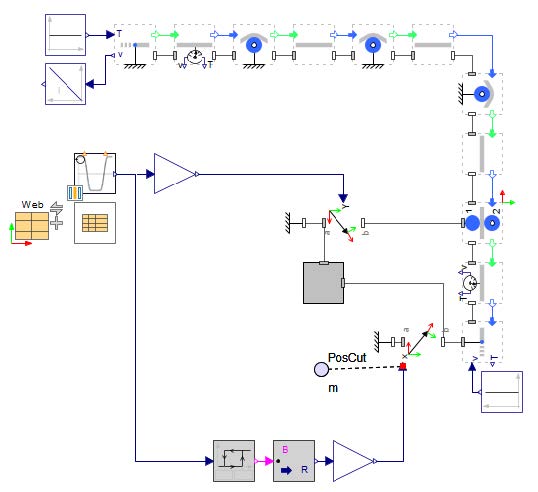
Figure 7.3: Structure of the model
Explore: Analyze the model structure, the referenced parameters for the stack definition and the motion profile.
The 3Dview and the front view is depicted in Figure 7.5. The motion axis and the end positions of the Nip Roller und the holding point is only for visualization purposes. This is modeled in the gray sub system of the model.
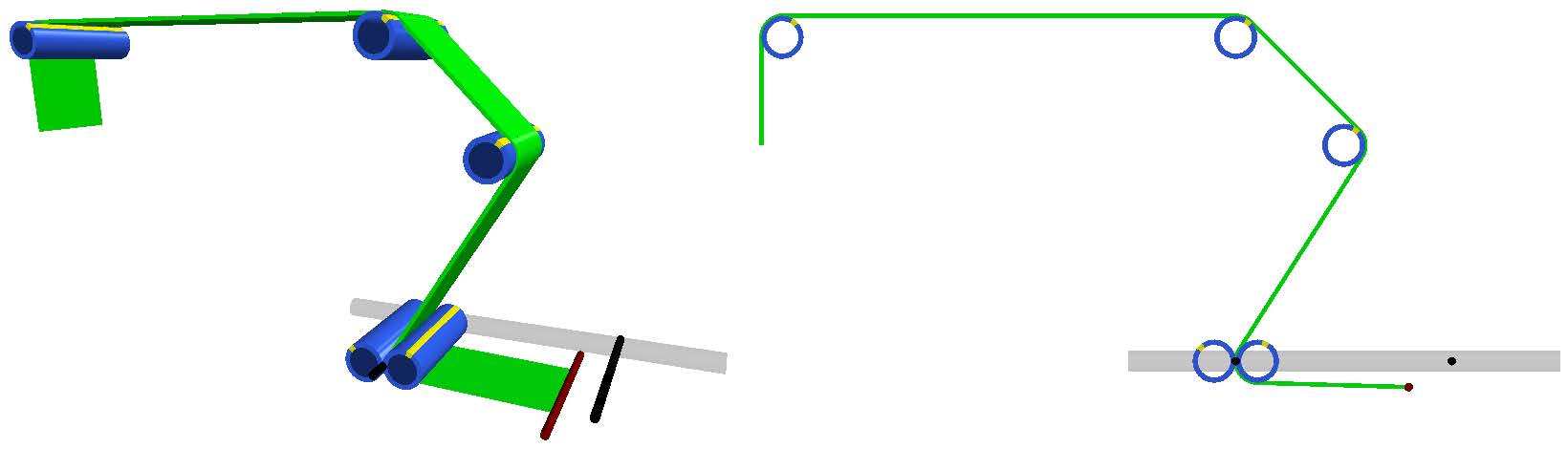
Figure 7.4: 3Dview and front view of the system
Figure 7.5 shows the simulation results. The first diagram (upper left diagram) presents the defined motion profile (red) from the 1D motion generation component which is multiplied by th half of the total motion distance LMove of the Nip Roller . The green curve is the switching position of the holding mechanism. The next diagram to the right shows the tensions of all spans and the next diagram to the right the tension of the stack span is presented. There are also 3 diagrams in the lower row. The first to the left shows the rotational speeds in [rad/s] of the Nip Roller . It can be observed how the rollers must be accelerate and decelerate during a folding cycle. The middle diagram contains the web speed of the Source and demonstrates that the in-going web must be moved back and forth into the tension zone of the z-Folding part. The last diagram is the integral of this speed and visualizes the total transported web length.
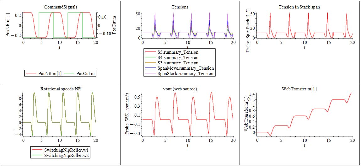
Figure 7.5: Simulation results
Download the model here zFolding02.msim and run the simulation (![]() )!
)!
The model is now extended with a master nip roller, a tension controlled linear dancer and a tension controlled unwinder. The model structure is shown in Figure 7.6. Figure 7.7 presents the 3Dview of the system. There are 2 load cells (brown rollers), a driven nip roller as master speed and a driven unwind drum. A driven linear dancer is used as a buffer to compensate the web motion based on the z-Folding.
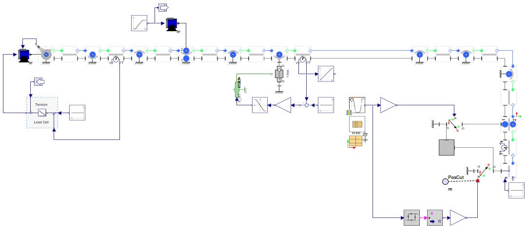
Figure 7.6: Structure of the model
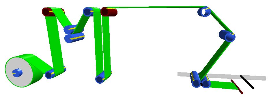
Figure 7.7: 3Dview
The results are presented in Figure 7.8. Besides the results of Figure 7.5 there are few new curves. The dancer position represents the dancer motion based on the tension control of the second load cell. The depicted reference web speed shows that the process has a continuous web speed from the unwinder to the linear dancer.
Figure 7.8: Simulation Results
It is possible to consider bearing losses for the rollers in a WH model. Normally it is not important and the most models can be used with zero bearing losses. But it is important to know the bearing losses working as resistances and influences the tension. This chapter demonstrate a use case where bearing losses are important.
Download the model here TestModelSlippage_ForwardMode_BearingLosses.msim and run the simulation (![]() )!
)!
Figure 7.9: Structure of the model
This model describes a tension zone of a web line with a very sensitive material which allows only a tension of 1N. The control structure is presented in Figure 7.10. The master drive defines the speed of the web line. The rotational dancer defines the reference tension point and is controlled by a tension controller. The load cell (brown roller) measures the tension as feedback signal. This means the tension controller calculates a torque signal for the rotational dancer to get the reference tension for the load cell. The second control loop is the position control for the entry nip roller of the tension zone. The task is to hold the rotational dancer in the zero position.
Figure 7.10: Control structure
Analyze the control structure and the parameter of the rollers! Question: Which behavior is expected?
The bearing losses are considered with the roller parameter d (bearing viscous damping constant). The assumed value is d = 6 · 10−6Nms/rad. This is a small but realistic value. The web speed is vweb = 2m/s and the idle rollers have a diameter of D = 24mm. With this web speed and roller diameter a loss torque of tauloss = 0.001Nm and a tension loss of Tloss = 0.083N can be calculated for each idle roller.
The Figure 7.12 shows the front view of the model where the web is colored by the tension value. The meaning of the color is the follow: Reference Tension, Zero Tension and Doubled Reference Tension. It can be seen that the tension goes down in direction of the left nip roller.
Why is the tension decreased? and Which behavior is expected if the machine runs in reverse mode?
Download the model here TestModelSlippage_ReverseMode_BearingLosses.msim and run the simulation (![]() )!
)!
Figure 7.11: Structure of the model
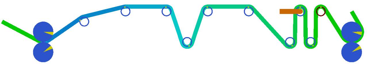
Figure 7.12: Tension behavior of the system in forward mode
In this model the machine direction is reversed and moves to the left. The Figure 7.12 shows the front view of the model with the same color setting than in the example before.
Why is the tension increased in this case? and How can the first model be changed to get the model in reverse mode?
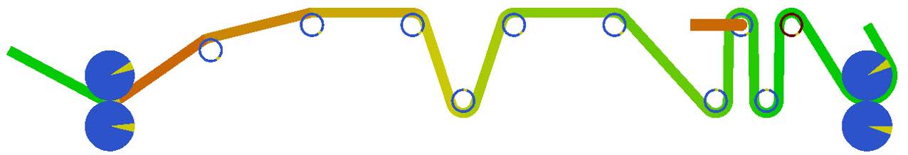
Figure 7.13: Tension behavior of the system in reverse mode
One use case of an R2R process is the separating of a web in different webs through slitting in machine direction. This section shows how this can be done in MapleSim and how this separated webs can be wound on different winder drums.
Download the model here SlittingAndWinding.msim and run the simulation (![]() )!
)!
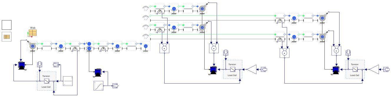
Figure 7.14: Model structure of the slitting and winding model
Figure 7.14 shows the diagram of the model. The process starts with an unwind drum which is tension controlled and uses a radius measurement. There is a driven nip roller to set the master web speed of the web line. After it the Slitter Roller is used to define 3 cutting points for the slitting in machine direction. The 3D view of the web line is depicted in Figure 7.15. It can be seen the 4 resulting webs are wound in pairs. In each case, 2 webs are wound onto one roll. This is modeled with the rigidly connected 1D rotational ports of the Wind Drum s. Each pair is tension controlled.
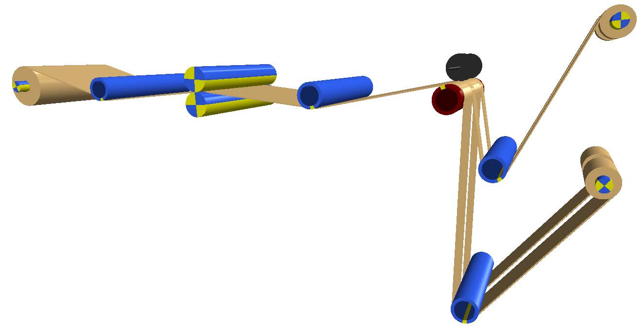
Figure 7.15: 3Dview
Analyze the model structure especially the wind drum configuration!
The Slitter Roller is parameterized similar to a classic Roller . There is an additional parameter section Settings to define the cut positions. It is shown in Figure 7.16. The slitting points are defined with respect to the far end of the web. The The seconds cut position cuts the web in the middle of it.
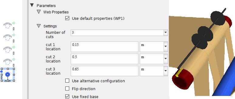
Figure 7.16: Parameters of the Slitter Roller
Analyze the cut parameters! Have a look on the help description.
This section demonstrates how the component Wind Drum Four Webs can be used to model and simulate the winding of anode, cathode and 2 separator lines in a production machine for cylindrical batteries.
Download the model here 4WebWinding.msim and run the simulation (![]() )!
)!
Figure Figure 7.17 presents the model structure which include the Wind Drum Four Webs and four subsystems for Separator 1, Cathode, Separator 2 and Anode. The main focus in this model are the web lines of Anode and Cathode. The web lines of the Separators are only implied. Figure Figure 7.18 shows the 3Dview of the model. Both web lines (Anode and Cathode) are driven by a nip roller and controlled with the position feedback of the dancer and a P-controller. The motion profile is defined with a component from the 1D-Motion-Generation-App. It describes the rotational speed of the mandrel.
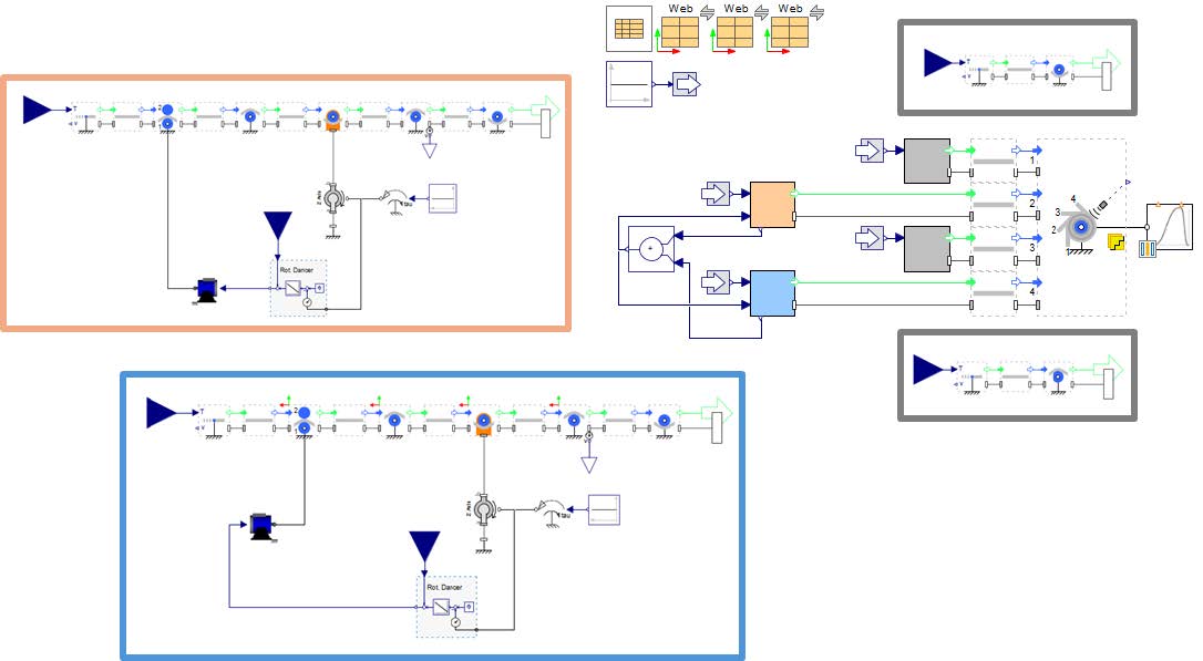
Figure 7.17: Model structure
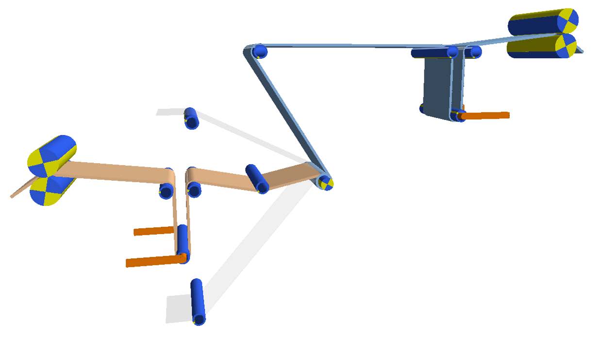
Figure 7.18: 3Dview
Analyze the model structure and discuss the following different simulations.
Simulate the model in the given parameterization!
Activate the feature "Use stepwise" in the component Wind Drum Four Webs and change the parameter "Merge angle web" δϕ to 180° Compare the results!
Activate the feature "Use multi-step" in the component Wind Drum Four Webs and change the following parameters:
ϕ4 = 0°,
ϕ4−>3 = 5°,
ϕ3−>2 = 15°,
ϕ2−>1 = 5°,
δϕ1 = δϕ2 = δϕ3 = δϕ4 = 100°, Compare the results!
The results are depicted in the following figures Figure 7.19, Figure 7.20 and Figure 7.21. All of them have the same structure. The upper row shows from left to right the diagram of the mandrel speed, the web speed of the Anode line and the web speed of the Cathode line. The lower row shows the Dancer angles, the turns of the mandrel and the web tension of the spans before the winding drum.
The mandrel wound 6 turn during this motion profile. The simulation shows an increased tension at the beginning during acceleration and a decreased tension of the mandrel decelerate. The dancers show a significant movement up to 8°. If the stepwise winding is activated an oscillation in the tension can be observed. This demonstrates how this feature can be used to analyze frequencies based on the winding. More detailed analyses allows the multi-step option.
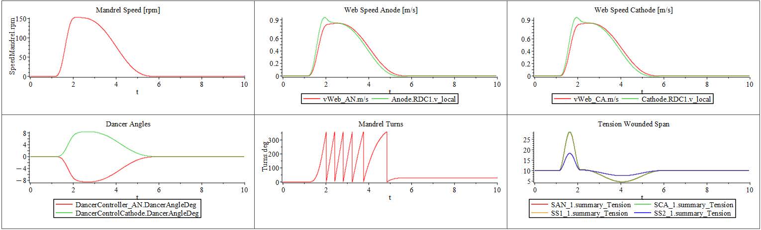
Figure 7.19: Results without stepwise winding
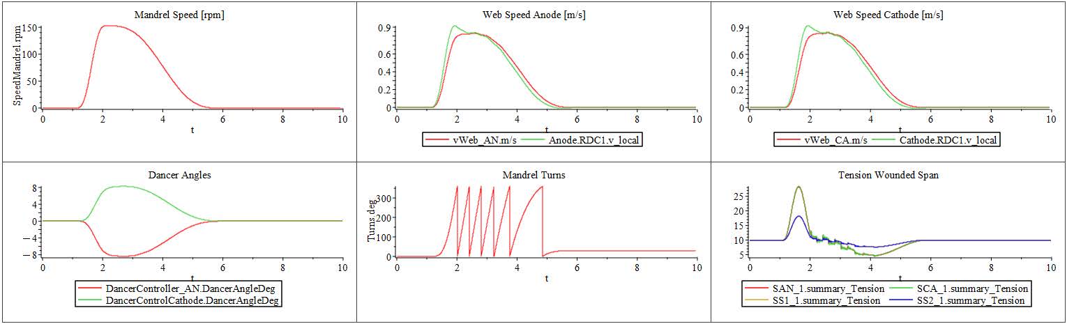
Figure 7.20: Results with single-step stepwise winding
Figure 7.21: Results with multi-step stepwise winding
Due to the web’s extremely thin nature relative to its width, it is highly susceptible to buckling when subjected to compressive stresses. One common cause of this behavior is the formation of troughs, which represent out-of-plane deformations occurring along a web span. At first glance, these troughs may appear harmless as they often move smoothly toward the next roller without causing immediate disruption.
However, these seemingly minor deformations can evolve into more severe issues downstream, particularly in the form of wrinkles. Wrinkles are a more pronounced and typically undesirable distortion of the web surface that often occur after the web passes through additional rollers or processes. This downstream wrinkling is generally a result of lateral compressive stress, and is often considered a worst-case scenario for a system.
The Trough Formation App in MapleSim is purpose-built to support the analysis and evaluation of trough formations in web handling systems. Specifically tailored for roll-to-roll (R2R) processes, this app allows users to closely examine the effects of out-of-plane web deformations, such as troughs or wrinkles. From this App a user can gain insight on the following;
Operational Conditions - Understanding the acceleration times, position and time setting for auxillary drives.
Roller Optimization - In regarding to the number ofrollers used, and effect of the bearing drag.
Tension set point.
Property of the web etc.
This example demonstrates the use of Trough Formation App in MapleSim.
Open the MapleSim model from Help > Examples > Web Handling App > Examples > Trough Formation Limit
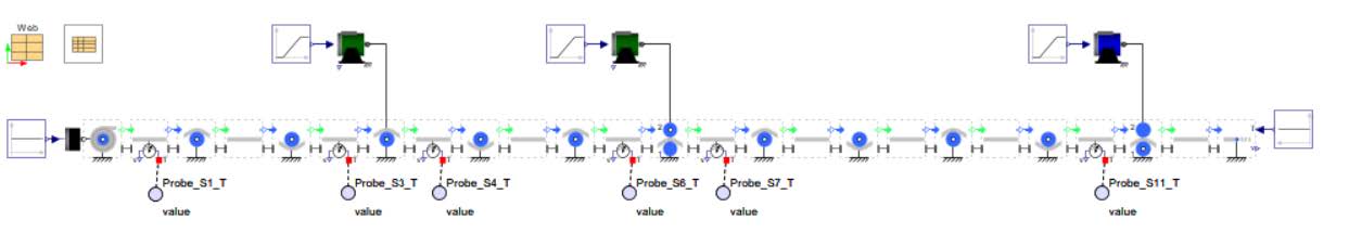
Figure 8.1: Example Model
Upon simulating the model, users can observe detailed results that illustrate the variation in tension across the web span, the master web speed, and the torque output of auxiliary drives throughout the process. In this specific setup, the model simulates the handling of a nonwoven web material, which is characterized by its soft, compliant nature. The primary driving element in this model is the right-side nip roller (NR1), which functions as the master drive. It governs the overall web speed and serves as the reference point for coordinating the motion of the other components in the system. In addition to NR1, the model includes two auxiliary torque drives strategically positioned along the web line. These drives are not responsible for setting the web speed but instead apply supplemental torque to fine-tune the tension distribution and support web transport.
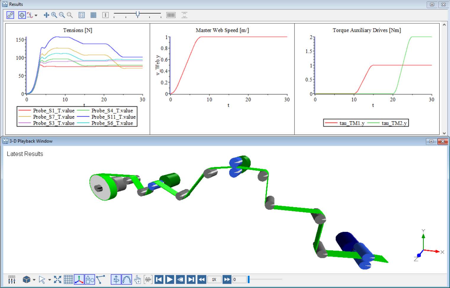
Figure 8.2: Model Results
Click ‘Add Apps or Templates’ (![]() ), then double click on the ‘Trough formation App’ from the Web handling section.
), then double click on the ‘Trough formation App’ from the Web handling section.
Figure 8.3: Selecting the Trough Formation App
Click ‘Load model’ under the configuration section of the App to load the MapleSim model into this App workspace.
Once loaded the clear message will pop up indicating that the model is loaded succesfully as shown below. The Properties of the web will also be populated in the respective fields.
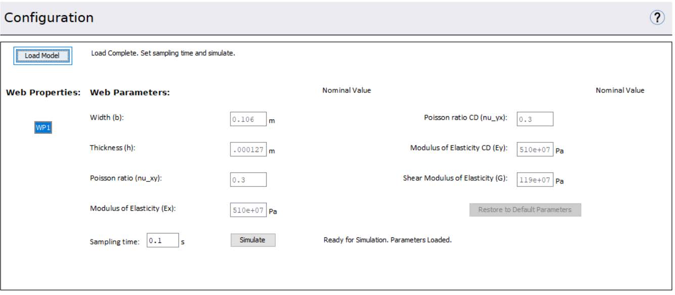
Figure 8.4: Loading the model in the App
The Web Property choose WP1 as this model contains only one preoperty block. If there are multiple web properties the user can choose from the list box.
The poissons ratio and poissons ratio CD cannot be 0.The value of poissons ratio CD defaults to the same value as the poissons ratio entered in the Web Property Block
Click on ‘Simulate’ to simulate the loaded model with the default parameters. Once simulation is complete, a clear message indicates the completion and all the parameter text boxes are now editable for the user to modify if needed for their analyses.
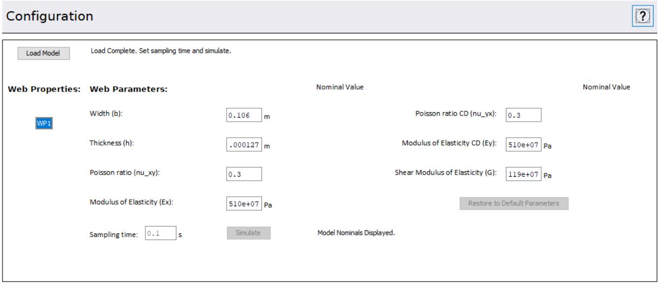
Figure 8.5: Parameters visible after simulation
The user can now click on any text box to change the parameters of the web and press ‘Enter’.
The first diagram shows the Misalignment Angle of each roller on the web line. The user has the option to choose individual spans or all from the List Box on the left.
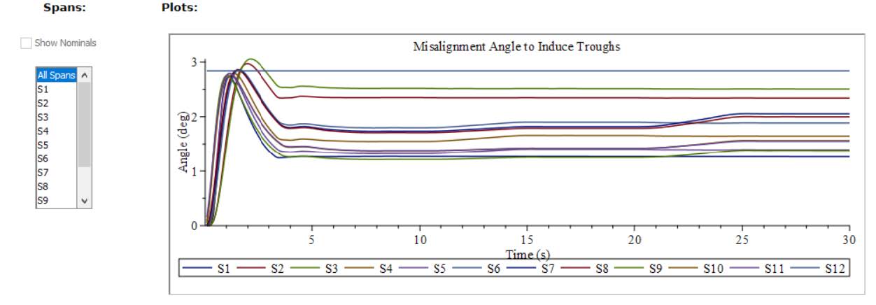
Figure 8.6: Misalignment angle of all spans
The second diagram shows the Web Trough Ratio Limit which is the evaluation about trough formation based on over tensioning.
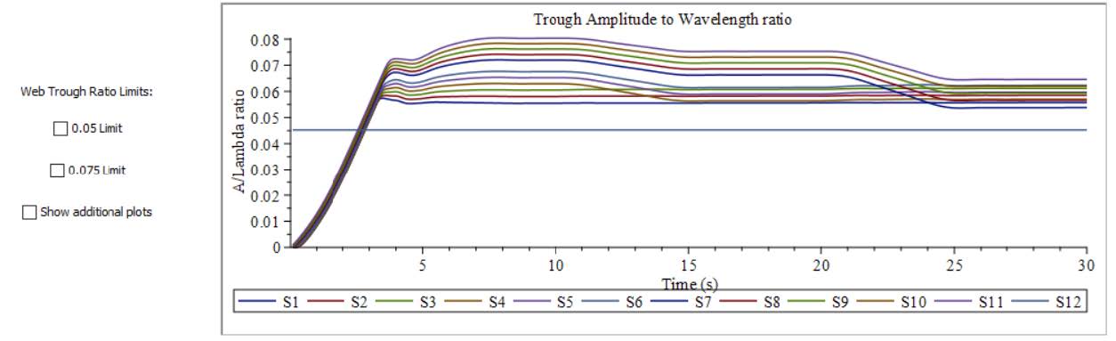
Figure 8.7: Web Trough Ratio plots
When the amplitude to wavelength ratio is greater than 0.05 and especially when its greater than 0.075, there is a greater risk for troughs to form based on research using finite elemnt modeling. By clicking on the ‘Web Trough Ratio limit’ options, the app plots its respective limits on the Web Trough Ratio plot.
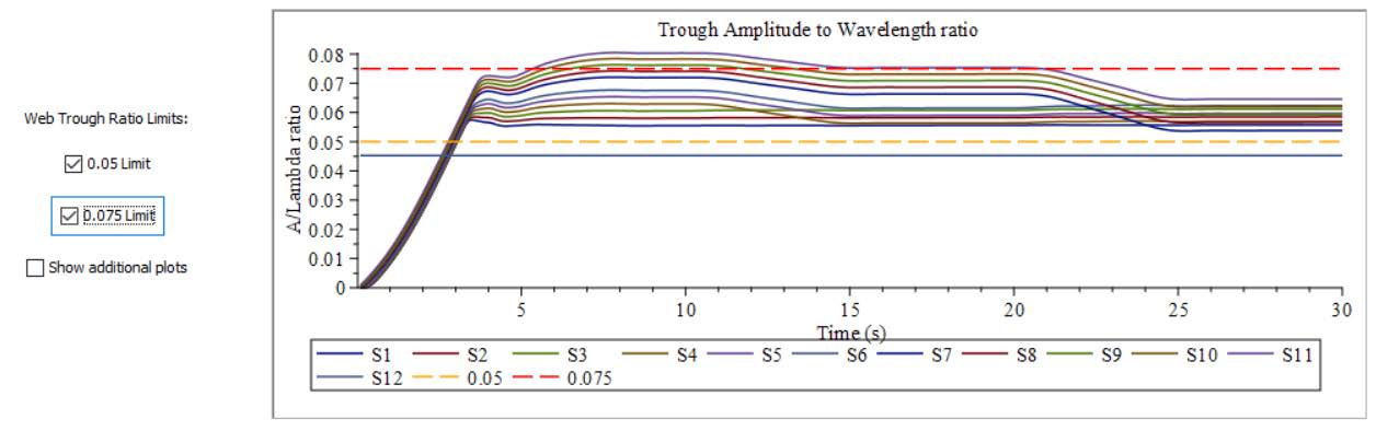
Figure 8.8: Web Trough Ratio Limit
Show additional plot options plots the amplitude of the troughs, wavelength of the troughs and the Tensions across the spans if needed.
The export option only allows to export data per span. When a span is chose, the plots can be exported to an excel file by clicking on the ‘Export Data’ button.
Figure 8.9: Export Options
The Parameter Sweep App in MapleSim allows the users to systematically explore and analyze how variations in model parameters affect system behavior. It enables users to define a set of parameters they wish to investigate and performs simulations across a range of specified values.
This is done efficiently by using compiled procedures, which significantly accelerates the computational process by allowing multiple simulations to be run in parallel, reducing the total time required for analysis.
As a result, the Parameter Sweep App is particularly well-suited for parameter sensitivity studies, design optimization where quick feedback on how parameter changes influence model outputs is essential.
In many roll-to-roll systems, a key challenge is managing the speed profiles of rollers throughout the system. In many cases the infeed rollers operate at or above the reference web speed to maintain adequate pulling force potentially could lead to web slacking. To address this, rollers downstream are intensionally driven at slightly lowe speeds than the nominal line speed. This speed offset introduces controlled tension in the web by creating a small stretch between rollers. The objective is to determine how variations in roller speed provided as a small percentage decrease from the reference speed affect the web tension profile. Lets take a simple MapleSim model to showcase the usability of this App.
This is a basic web line model designed to analyze how variations in speed affect the tension within the web. This model is designed purely to showcase the usage of the App.
Figure 8.10: Simple Web Line Example
On simulating the model we can now see the tension on the upstream section of Roller 3 as shown below. Since the speed is constant throughout the system reaches steady state and attains the tension set point.
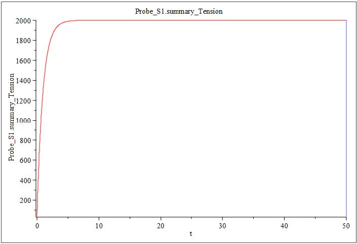
Figure 8.11: Simple Web Line Example
If we look closely in the Ramp component we notice that the increase of speed of the roller R3 is parameterized with value k. Now this is originally set to zero in the model to showcase that the system is running at the same speed. As an exercise we are now going to sweep through this parameter to see the influence of the downstream tensions due to the change in the speed.
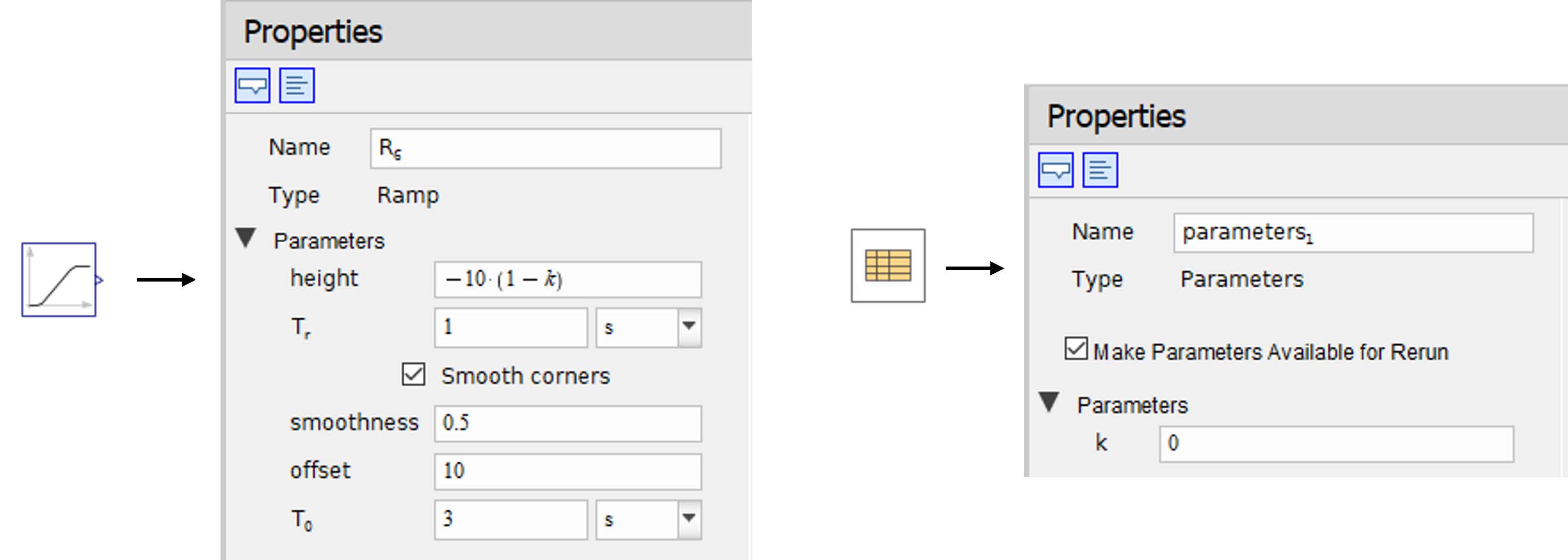
Figure 8.12: Parameter Set-up
Click ‘Add Apps or Templates’ (![]() ), then double click on the ‘Parameter Sweep App’ by expanding through ‘Model Analaysis’ section.
), then double click on the ‘Parameter Sweep App’ by expanding through ‘Model Analaysis’ section.
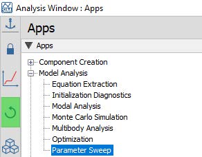
Figure 8.13: Open Parameter Sweep App
In the app, click on the ‘Load System’ button. This links the app to the current model and imports all the model information for use in the app. If changes are made to the model then this button needs to be re-clicked to import all the changes into the app.
Under the Configuration section click on the dropdown box to choose the parameter ‘k’ and click on ‘Add’
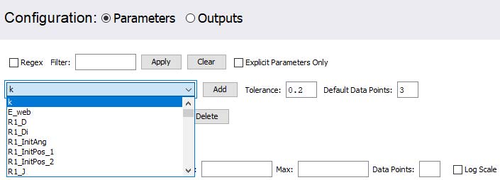
Figure 8.14: Add Parameter
Choose the limits and number of datapoints for the simulation as when below
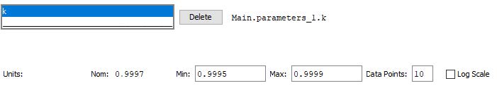
Figure 8.15: Add Parameter value range
Select the ‘Output’ radio button. Under this option the user can choose which outputs to analyze and the plots to see.
Select the ‘Last Point’ option as shown below for Span 1 Tension.
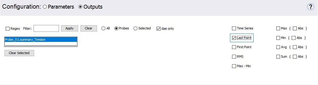
Figure 8.16: Output options
The ‘Last Point’ option enables users to extract only the final value from each simulation run. In this particular analysis, since the system reaches a steady state, our primary interest lies in the steady-state tension value of Span 1. Therefore, selecting the "Last Point" setting is appropriate, as it efficiently captures the relevant data once the system has settled.
Under the Execute Para,eter Sweep option click on ‘Run Parameter Sweep’ to run the simulations.
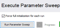
Figure 8.17: Run Sweep
Once the simulations are complete now choose ‘k’ under the Param 1 option which shows the parameter variation in the x-axis. The y axis shows the LAst Point Tension value for each simulation.
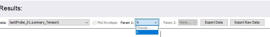
Figure 8.18: Results Display setting
The results now illustrate how variations in speed affect the tension in Span 1.
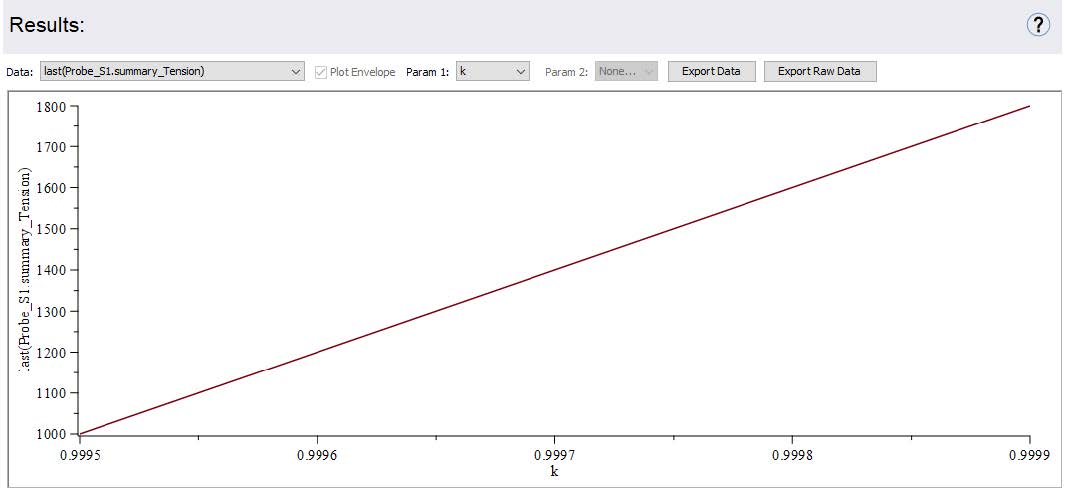
Figure 8.19: Tension variation due to speed changes
The purpose of this exercise is to demonstrate how the Parameter Sweep App can be effectively used to quickly analyze the impact of varying parameters on system behavior. By using compiled procedures, the app significantly accelerates the simulation process, enabling multiple runs in a short amount of time—far more efficiently than manually adjusting parameters and running individual simulations within the MapleSim environment.
The 1D Motion Generation App is a specialized tool designed to help users create custom or unique motion profiles that can be used to control various parts of a dynamic system. These motion profiles define how a component (e.g., a slider, actuator, or rotary joint) moves over time and are essential in applications where specific displacement, velocity, acceleration, or jerk constraints must be met. While it is technically possible to construct such motion profiles using the standard Signal Blocks library in MapleSim by combining basic building blocks such as ramps, step signals, sine waves, or polynomial equations this approach can quickly become tedious for more complex motion requirements.
For this exercise we are going to take an accumulator example model and define custom entry and exit speeds of the web line. This model demonstrates how an accumulator is modeled in MapleSim. The accumulator is designed to temporarily store web material to manage tension variations and compensate for speed mismatches between the upstream and downstream processes.
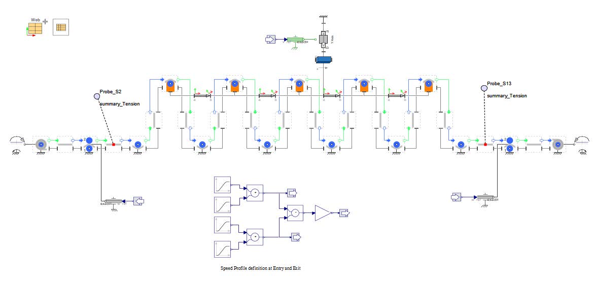
Figure 8.20: Accumulator model
The model features both a wind drum and an unwind drum, each with a constant torque input.
Two nip rollers, one at the entry and one at the exit of the accumulator, regulate the web speed entering and leaving the accumulator. These rollers are driven based on pre-defined speed profiles.
The accumulator structure includes a carriage that moves vertically to store or release web material. The model is configured with 10 spans of web between fixed and movable rollers on the carriage, representing the capacity of the accumulator.
The speed of the carriage is not defined, but it is calculated based on the difference between the entry and exit web speeds. When the entry speed is greater than the exit, the carriage moves upward to store more web. Conversely, if the exit speed is higher, the carriage moves downward to feed material into the downstream section.
In this chapter we are going to define a custom speed profiles for entry and exit using the 1D motion generation App instead of the Ramp signals that are originally used.
Click ‘Add Apps or Templates’ (![]() ), then double click on the ‘1D Motion Generation App’ by expanding through ‘component Creation’ section.
), then double click on the ‘1D Motion Generation App’ by expanding through ‘component Creation’ section.
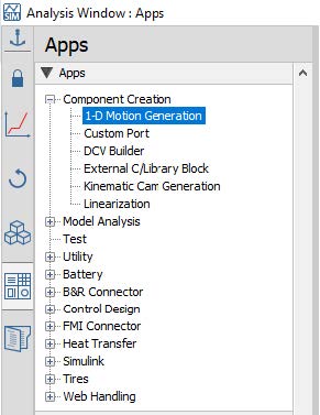
Figure 8.21: Selecting the App
You can choose to add as many as axes you want in this section. Each of these axes will be a signal output port for the generated component. Also, you can use arrow buttons to change the order of the axes and (+/-) buttons to add a new one or delete the selected axis. In this section we are going to create two motion profiles, one for entry and other for exit. For now we will start with a single axis and create the entry speed.
This section of the app allows the user to specify the properties of an axis. You can change the axis name, offset, and the type of the output port. The output port can be Translational, Rotational Angle, Rotational Velocity, or a Signal port. The default units for the profile variables can be also changed using the drop-downs.
The entry speed starts at 10 rad/s for 50 seconds and decelerates to 0 within a period of 10 seconds before accelerating back to 10 rad/s.
Rename the signal name to Entry, and set the offset to 10.
Select ‘Signal’ from the ‘Type’ drop-down menu in this section.
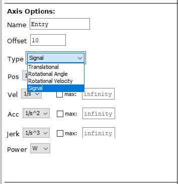
Figure 8.22: Selecting the type of signal
The signal is defined for 1 second which can be seen in preview. Lets adjust the time of the signal to 50 seconds for a constant speed of 10. To do that we are going to change the duration of the signal to 50. You can now notice th signal has now changed to 50 [sec]
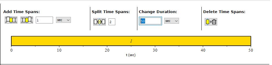
Figure 8.23: Change the duration
Lets now move on to the second part of the signal where the speed drops to 0 in a duration of 10 [sec]. To do that lets first add an additional 10 seconds to the motion by using the Add Time Spans section. We can now see an additional 10 seconds added to the waveform.
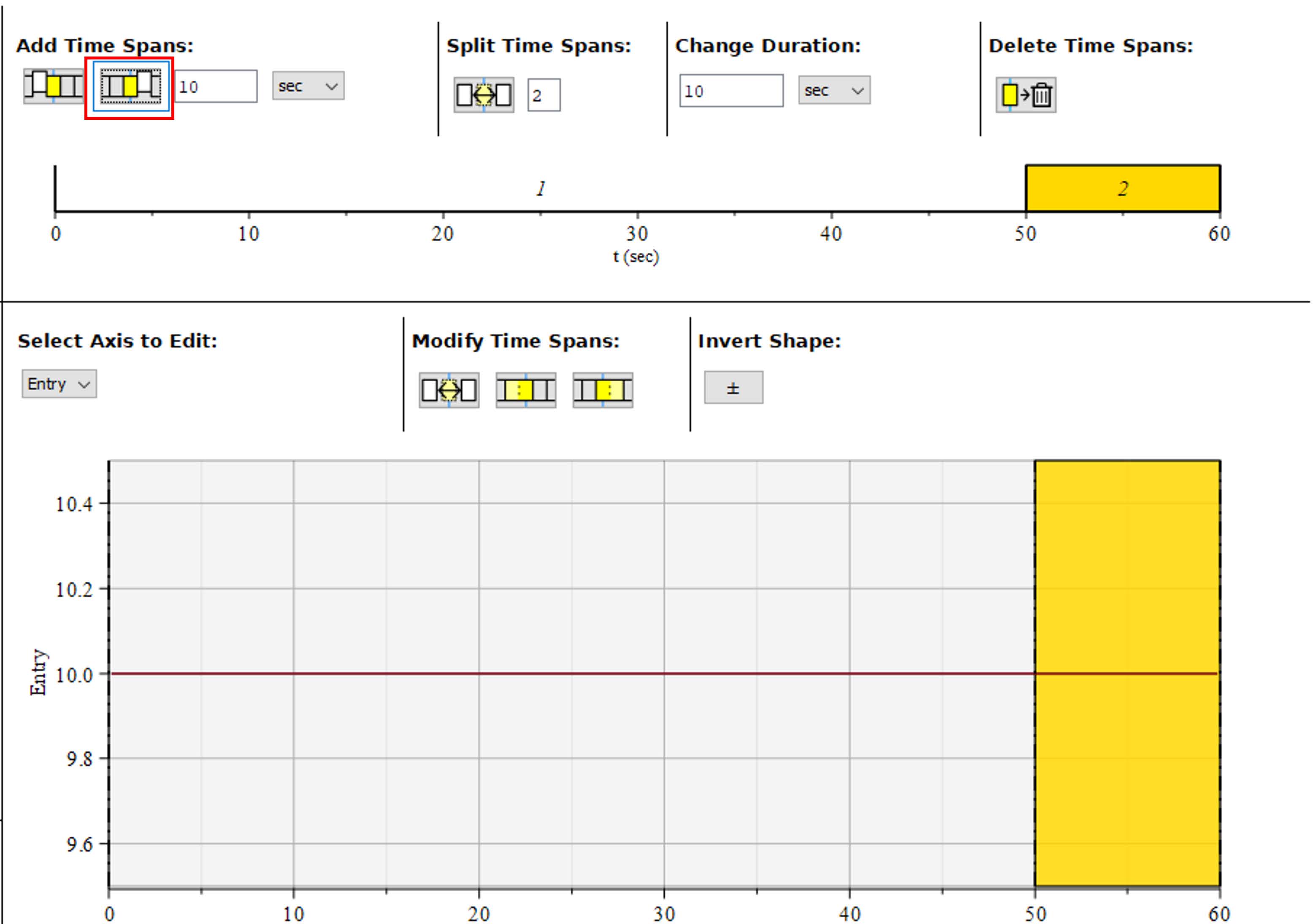
Figure 8.24: Adding Duration
To create the waveform of the motion profile, user needs to define the time span and set the ‘Segment Options’ properties such as ‘Shape’ and ‘Height’ for the selected time span (highlighted in yellow). The option from the profile drop down menu allows the user to select the type of shape of the selected segment. Available options for the profile shape are
Lets add Bestehorn curve and set the height to -10 and press Enter. When we press enter the shape reflects on the waveform.
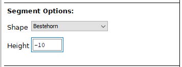
Figure 8.25: Set the shape type and height
Now lets add the last part of the ramp by where the speed increases back to 10 in a duration of 10 [sec]. To do that lets first add an additional 10 seconds to the motion by using the Add Time Spans section. We can now see an additional 10 seconds added to the waveform.
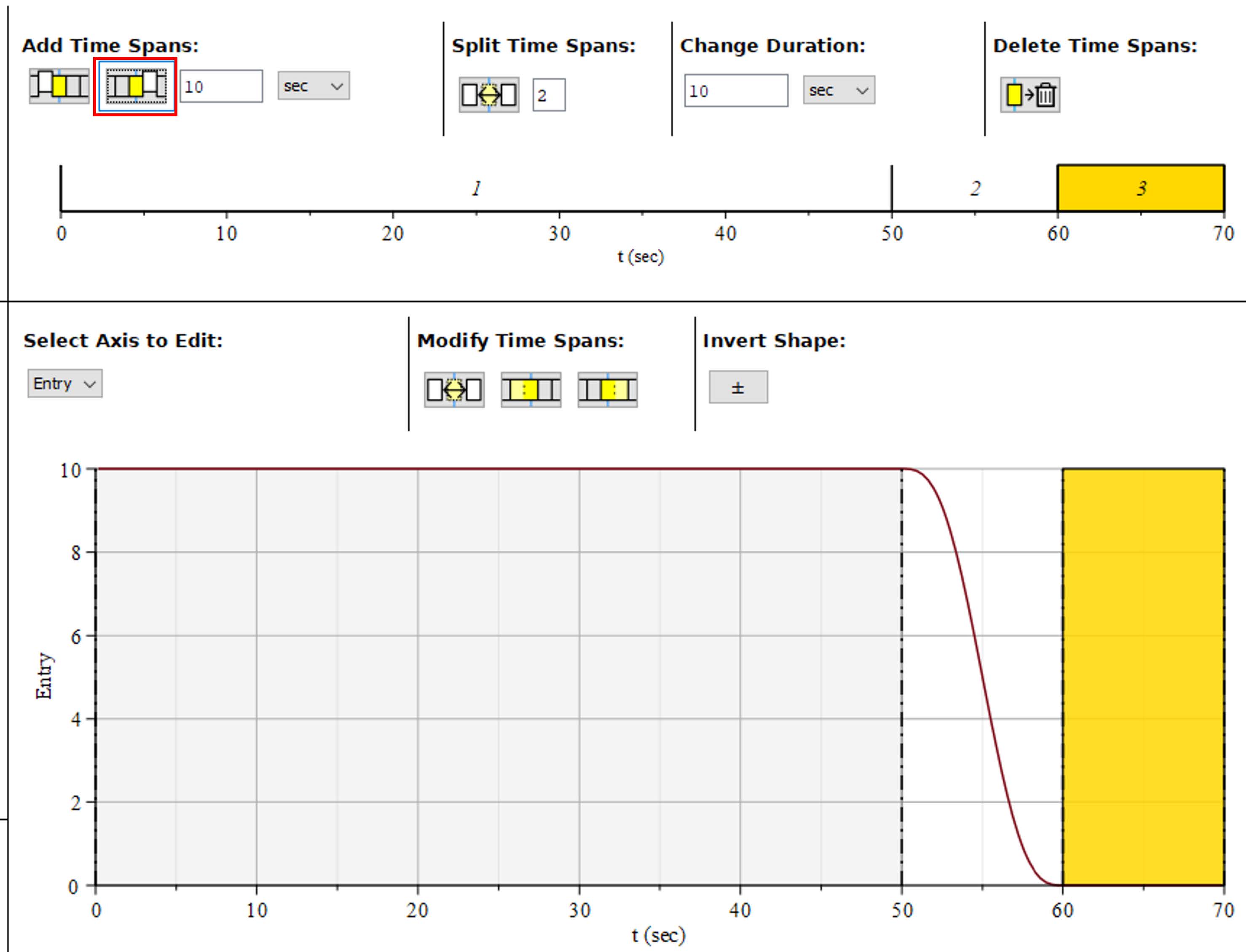
Figure 8.26: Adding additional duration
Lets add Bestehorn curve and set the height to 10 and press Enter. When we press enter the shape reflects on the waveform.
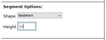
Figure 8.27: Adding the shape type and height
The entry waveform is now complete.
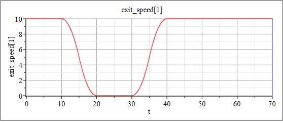
Figure 8.28: Exit Speed
Lets add an additional axis now by clicking on the (+) sign under the Axes option.
Figure 8.29: Exit Speed Axes
Rename the signal now to Exit. Make sure that the second axis is selected under the Axes section. This allows the user to know which waveform the user is currently editing.
The App automatically assigns the previous waveform to this new profile as well., Now the user has multiple ways to approach this by using the options. However for this exersice lwts use the most direct option which is to delete the existing waveform by selecting the Delete waveform option twice.
Figure 8.30: Delete existing span
Lets change the duration of first waveform to 10 [sec] instead of 50.
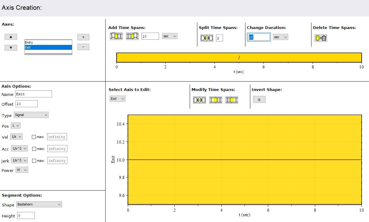
Figure 8.31: defining the first section of profile
Lets now move on to the second part of the signal where the speed drops to 0 in a duration of 10 [sec]. To do that lets first add an additional 10 seconds to the motion by using the Add Time Spans section. We can now see an additional 10 seconds added to the waveform.
For the selected part of waveform add Bestehorn curve and set the height to -10 and press Enter. When we press enter the shape reflects on the waveform.
Now again add part where the speed remains constant to 0 in a duration of 10 [sec] by using the Add Time Spans section. We can now see an additional 10 seconds added to the waveform.
if we look into the original curve we see now the waveform gains to 10 after 30 seconds. So Lets add another 10 [sec] by using the Add Time Spans section.
For the selected part of waveform add Bestehorn curve and set the height to 10 and press Enter. When we press enter the shape reflects on the waveform.
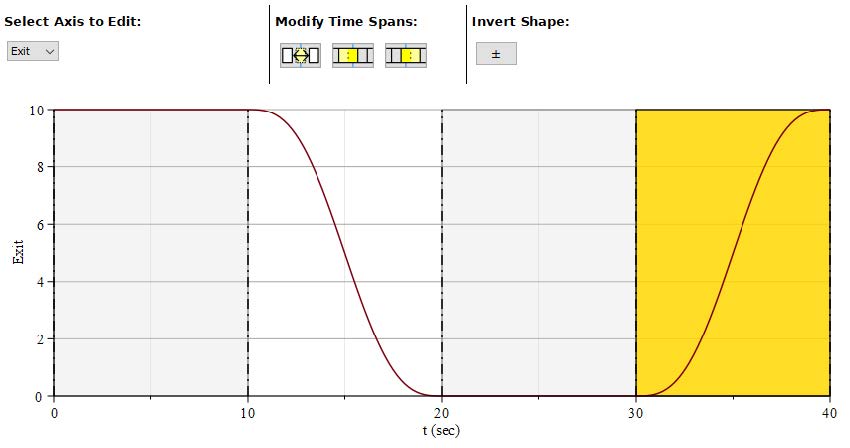
Figure 8.32: defining the rest of the profile
The last part of the waveform is constant at 10 for 30 [sec] . so lets add a 30 [sec] time span by using the Add Time Spans section and complete the waveform.
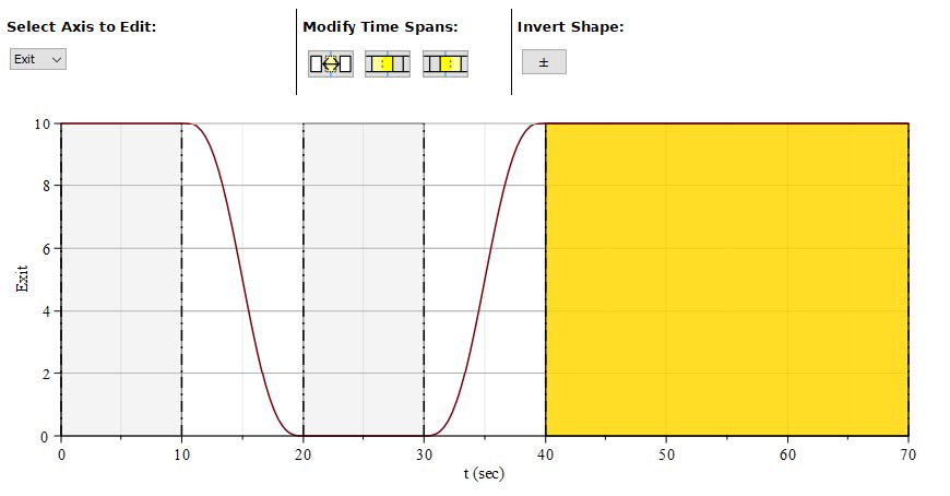
Figure 8.33: Final waveform
Now we can generate the profile by scrolling under the Model Generation section and creating a new component name and selecting Generate
Figure 8.34: Creating the component
You can find the generated component under the ‘Local component’ section in MapleSim.
Figure 8.35: Local Component section
You can now drag the component and replace the ramp signals with the new motion profile as shown below and ‘Simulate’ to generate the model and see the results.
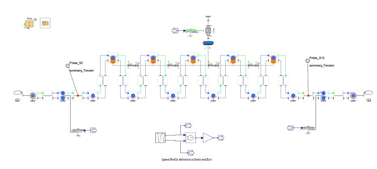
Figure 8.36: Final model